Basic unmixing example

This tutorial documents the interactive script user_scripts/unmix_example.py. It is the best starting point for learning the core unmix(...) workflow on a simple two-channel example.

How to use this tutorial

The script is designed to be run as an interactive Python script, best with an IDE that supports cell-based execution (e.g., Spyder, VSCode, or PyCharm).

It is organized in cells, reflecting the structure of this tutorial. Thus, the recommended way to follow this tutorial is:

1. download and open the user_scripts/unmix_example.py script,

2. run the cells from top to bottom,

3. adjust the configuration values that are relevant for your own data.

The subsections below follow the same order as the script cells.

What this tutorial covers

The script demonstrates:

• fixed-alpha correction,

• reference-time-point alpha estimation,

• several automatic alpha-estimation methods,

• and direct napari inspection after each run.

Imports

The first cell imports the package functions used throughout the tutorial.

The most important imported helpers are:

• unmix(...) as the core workflow,

• report_path_from_output_path(...) to inspect the JSON sidecar,

• show_unmixed_channels_in_napari(...) to visualize the result.

from __future__ import annotations

from pathlib import Path

PROJECT_ROOT = Path(__file__).resolve().parents[1]

from spectral_unmixing import (
    report_path_from_output_path,
    show_unmixed_channels_in_napari,
    unmix)

Note

PROJECT_ROOT = Path(__file__).resolve().parents[1] is used to locate the example dataset and output directory relative to the project root. You can change this to a fixed path if you want to run the script from a different working directory. You can completely remove this line if you want to use absolute paths for input and output (see the next cell).

Define input and output paths

Next, we need to define the input dataset and the output filenames used by the examples:

INPUT_PATH = PROJECT_ROOT / "example_data" / "PICASSO_examples" / "2_color_unmixing_validation.tif"
INPUT_NAME = INPUT_PATH.stem
OUTPUT_DIR = INPUT_PATH.parent / "unmixed"
OUTPUT_DIR.mkdir(parents=True, exist_ok=True)
# %% OPTIONAL: INSPECT PREPARED STACKS IN NAPARI
from spectral_unmixing.viewer import show_all_channels_in_napari
show_all_channels_in_napari(INPUT_PATH, layer_prefix="2-channel example")

What you can change here:

• INPUT_PATH to point to a new OMIO-readable microscopy stack, and

• the output directory or naming scheme.

Spectral unmixing with a manually set alpha

The first cell in the script demonstrates the usage of a user-provided, fixed alpha value for the full stack. This is the simplest and often most scientifically interpretable mode when a coefficient has been measured from a suitable control dataset or has been determined from prior knowledge.

The corresponding cell consists of three main steps:

1. set an OUTPUT_PATH (here called OUTPUT_FIXED) for the corrected stack,

2. call unmix(...) with the fixed alpha,

3. visualize the result in napari using show_unmixed_channels_in_napari(...).

OUTPUT_FIXED = OUTPUT_DIR / f"{INPUT_NAME}_unmixed_fixed_alpha.tif"

fixed_output = unmix(
    input_path=INPUT_PATH,
    output_path=OUTPUT_FIXED,
    # source_channel=0,  # default: 0
    # target_channel=1,  # default: 1
    method="manual",
    alpha=0.62,
    # alpha_mode="fixed",  # only relevant for multi-time-point stacks; default: None; other options: "reference_t", "per_t"
    # clip_negative=True,  # default: True
    # output_dtype="float32",  # default: "float32"
    # verbose=True,  # default: True
)

show_unmixed_channels_in_napari(
    fixed_output,
    source_channel=0,
    target_channel=1,
    layer_prefix="Fixed alpha",
    source_colormap="cyan",
    target_colormap="yellow")

The important knobs are:

• method="manual": tells the workflow to use a user-provided alpha value instead of estimating one from the data.

• alpha: manually supplied bleed-through coefficient. Larger values subtract more source signal from the target channel; smaller values leave more residual bleed-through behind.

• alpha_mode="fixed": keeps that same alpha for the whole stack. This is mainly relevant when the data have multiple time points. You can also leave alpha_mode unset or pass None here, because None is the default and the pipeline will internally resolve to fixed whenever method="manual" is used together with a user-provided alpha.

• optional source_channel and target_channel: define the direction of correction. Changing them changes which channel is treated as the contaminating source and which one is corrected.

• optional clip_negative: if enabled, negative corrected intensities are clipped to zero after subtraction.

• optional output_dtype: controls the precision used for the written result. float32 is the sensible default for most workflows.

• optional verbose: enables or suppresses terminal progress output and parameter reporting.

• optional visualization colormaps for napari

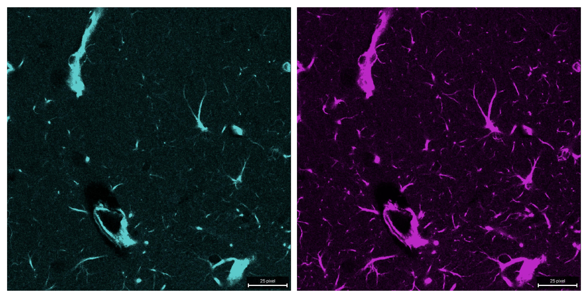
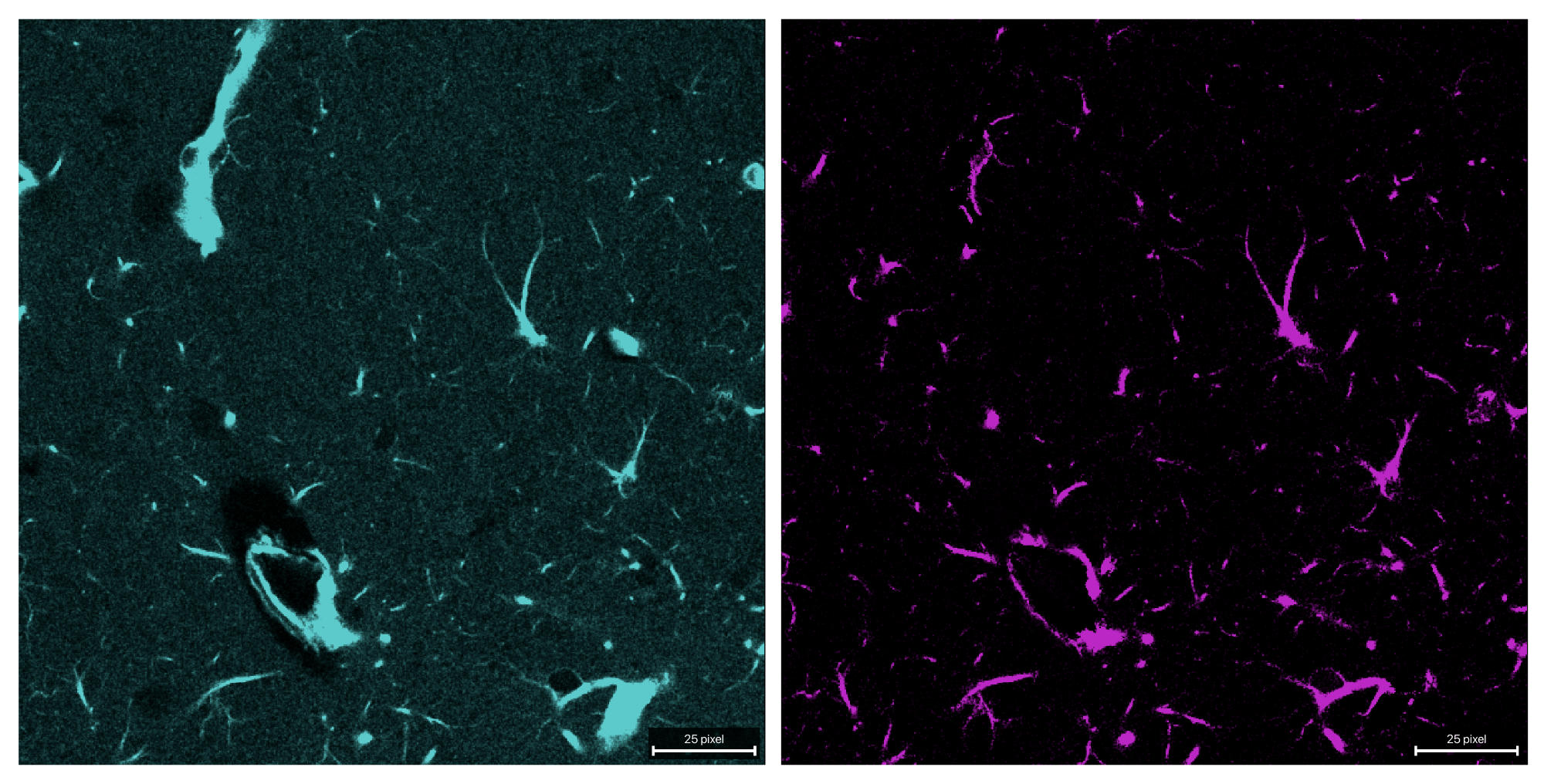
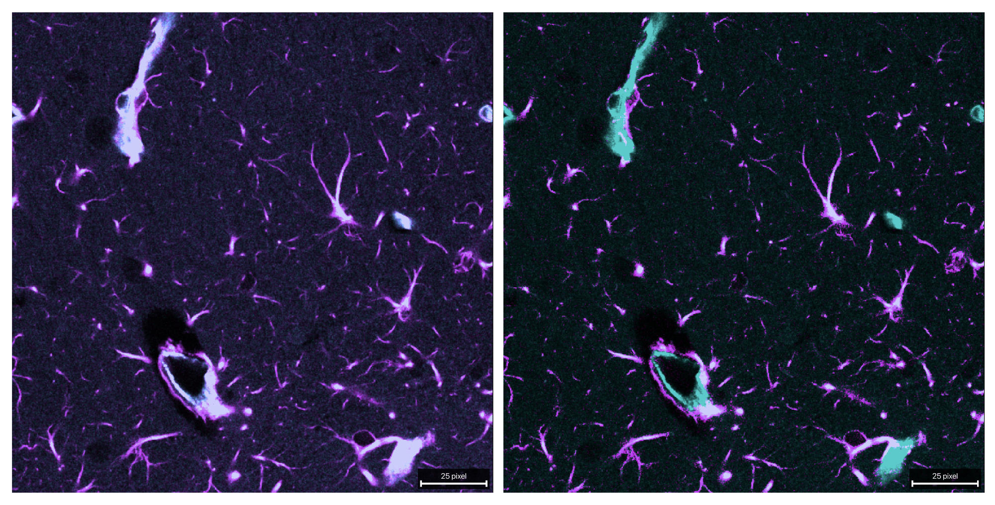
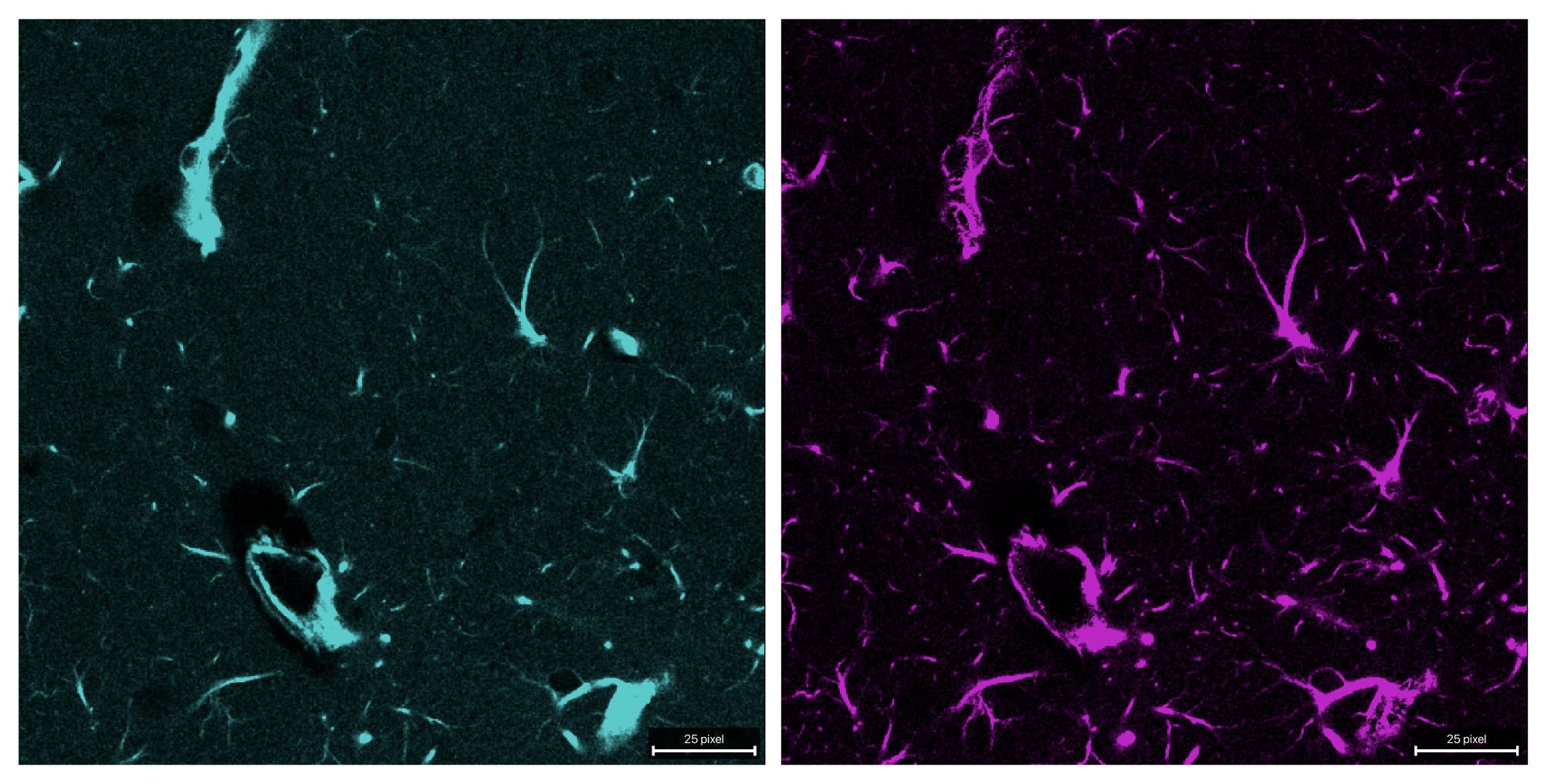
The raw two-channel example stack used in this tutorial. Channel 0 (cyan) bleeds into channel 1 (magenta) and is thus the source channel. Channel 1 is the target channel that we want to correct.

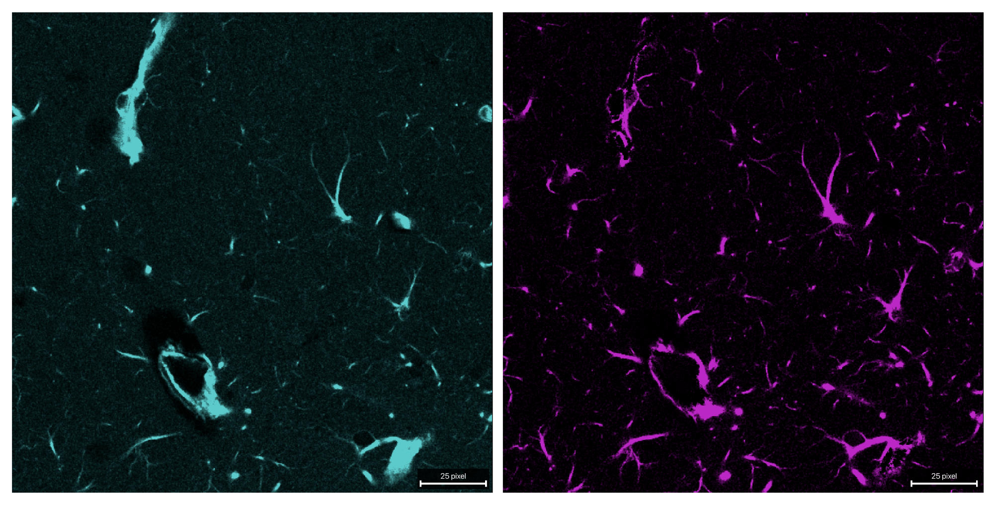
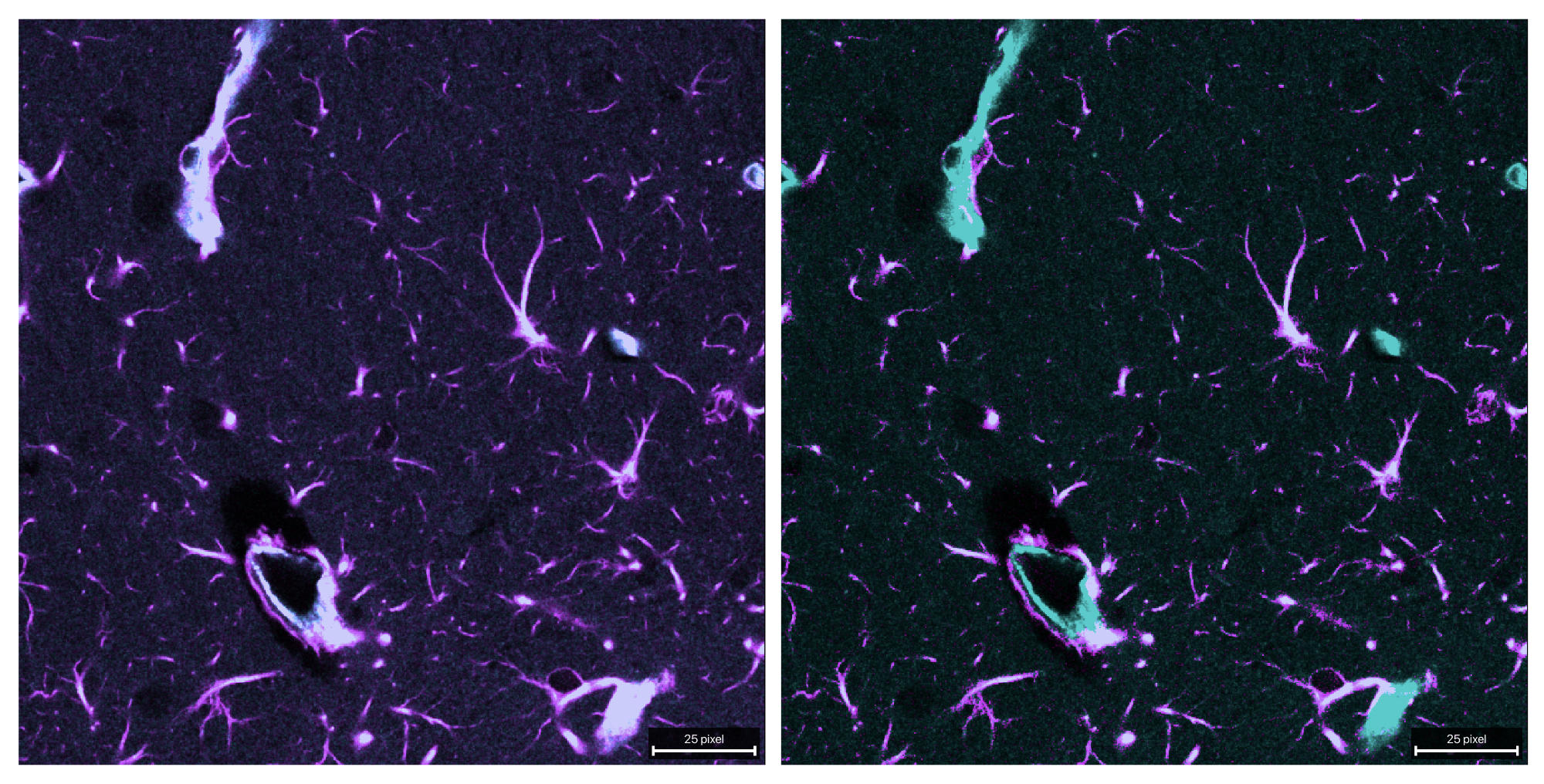
Both channels after unmixing with a fixed alpha of 0.62. The bleed-through from channel 0 into channel 1 is largely removed, while the original signal in channel 1 is preserved.

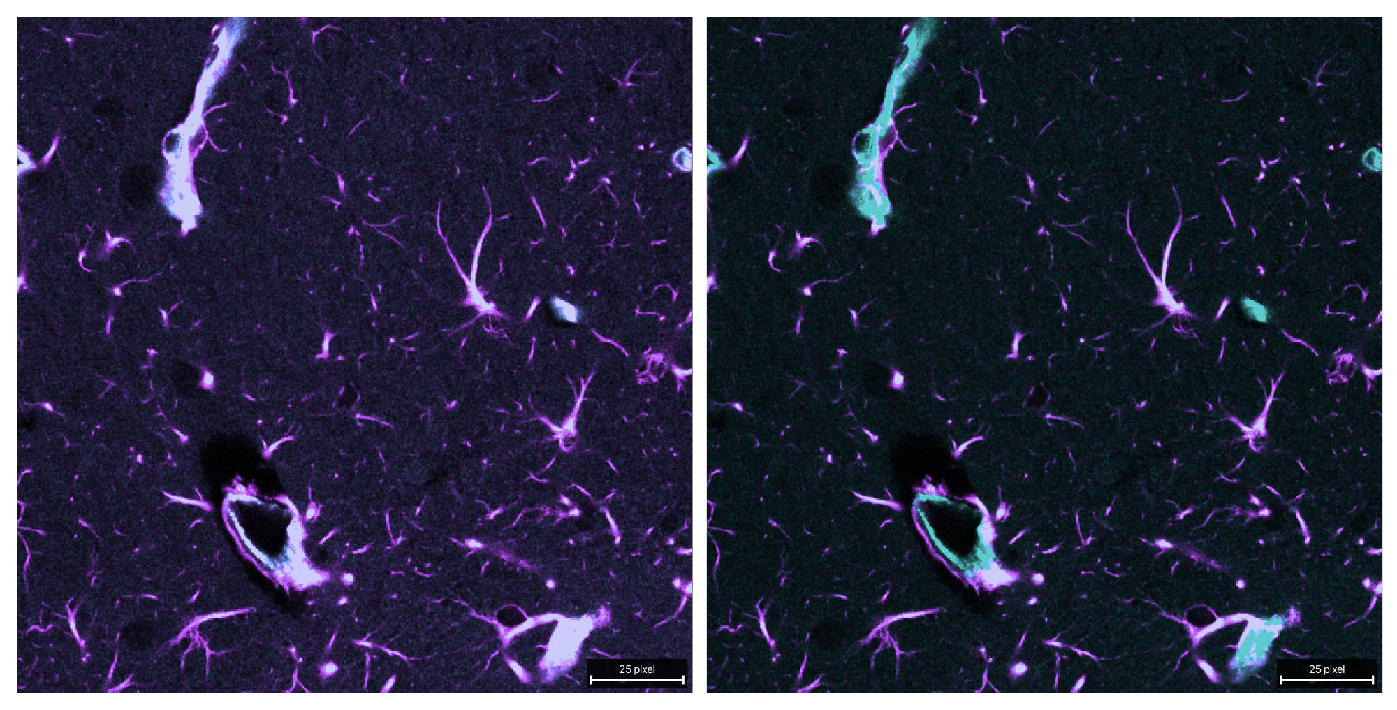
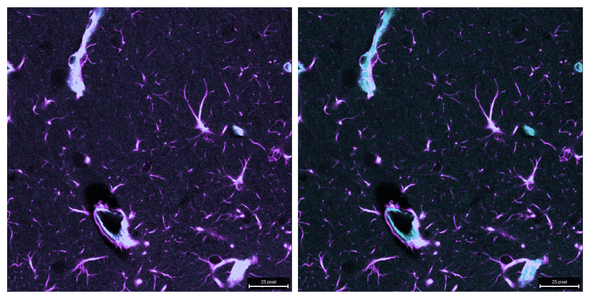
Composite comparison of the raw (left) and unmixed (right) stack. The bleed-through from channel 0 into channel 1 is clearly visible in the raw data, while it is largely removed in the unmixed result and, thus, a more accurate representation of the true signal in channel 1 is obtained.

mean_ratio method

By changing the method to mean_ratio, alpha is computed as the mean target intensity divided by the mean source intensity within a mask that is defined by the signal_percentile and background_percentile parameters:

OUTPUT_REFERENCE = OUTPUT_DIR / f"{INPUT_NAME}_unmixed_reference_t0_mean_ratio.tif"

reference_output = unmix(
    input_path=INPUT_PATH,
    output_path=OUTPUT_REFERENCE,
    # source_channel=0,  # default: 0
    # target_channel=1,  # default: 1
    method="mean_ratio",
    #alpha_mode="reference_t",
    #alpha_reference_t=0,
    signal_percentile=99.0,
    background_percentile=1.0,
    # target_low_percentile=95.0,
    # preprocess_alpha_inputs=True,  # default: True
    # clip_negative=True,  # default: True
)
print(reference_output)
print(report_path_from_output_path(reference_output).read_text(encoding="utf-8"))
show_unmixed_channels_in_napari(
    reference_output,
    source_channel=0,
    target_channel=1,
    layer_prefix="mean_ratio")

Important parameters:

• method="mean_ratio": estimates alpha as the ratio of mean target and mean source intensity inside the selected source-dominant mask.

• signal_percentile: defines how strict the bright-source mask is. Higher values keep only the brightest source voxels and make the estimate more selective; lower values include more voxels but may mix in less source-specific regions.

• background_percentile: defines the low-percentile background level that is subtracted before alpha estimation. Increasing it removes more low-intensity baseline; decreasing it keeps more of the original dim signal.

• optional target_low_percentile: further restricts the estimation mask to comparatively dim target voxels. Lower values make this restriction stricter; higher values relax it.

• optional preprocess_alpha_inputs: switches the percentile-based background subtraction and clipping used only for alpha estimation. Turning it off makes the estimate depend more directly on the raw measured intensities.

• alpha_mode and alpha_reference_t: become relevant for real multi-time-point stacks. reference_t estimates one alpha from the selected reference time point and applies it to all time points. The same mean_ratio estimator can also be combined with alpha_mode="per_t" when you want one separately estimated coefficient per time point. Please refer to the dedicated multi-time-point tutorial Full 3D+t unmixing example for more details on that workflow.

Increasing signal_percentile makes the mask more selective. Lowering it uses more voxels but may mix in less source-specific regions.

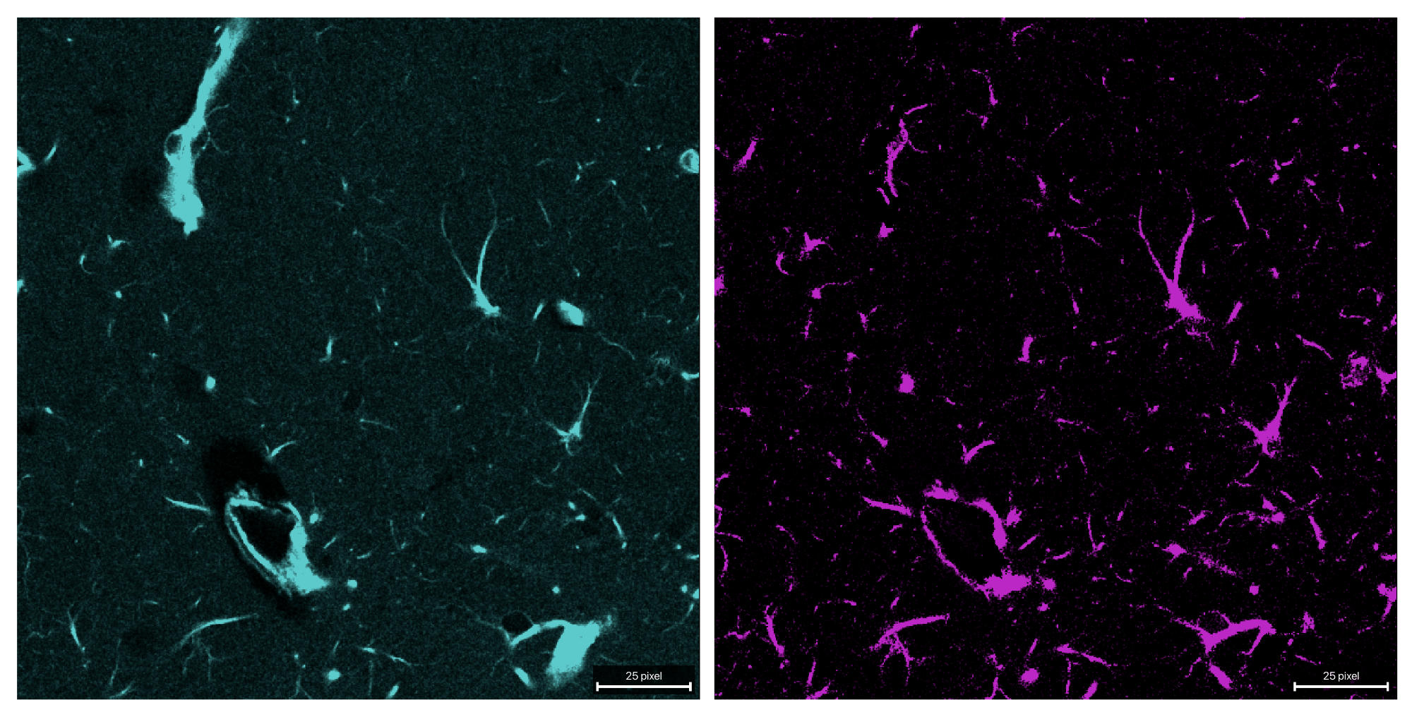
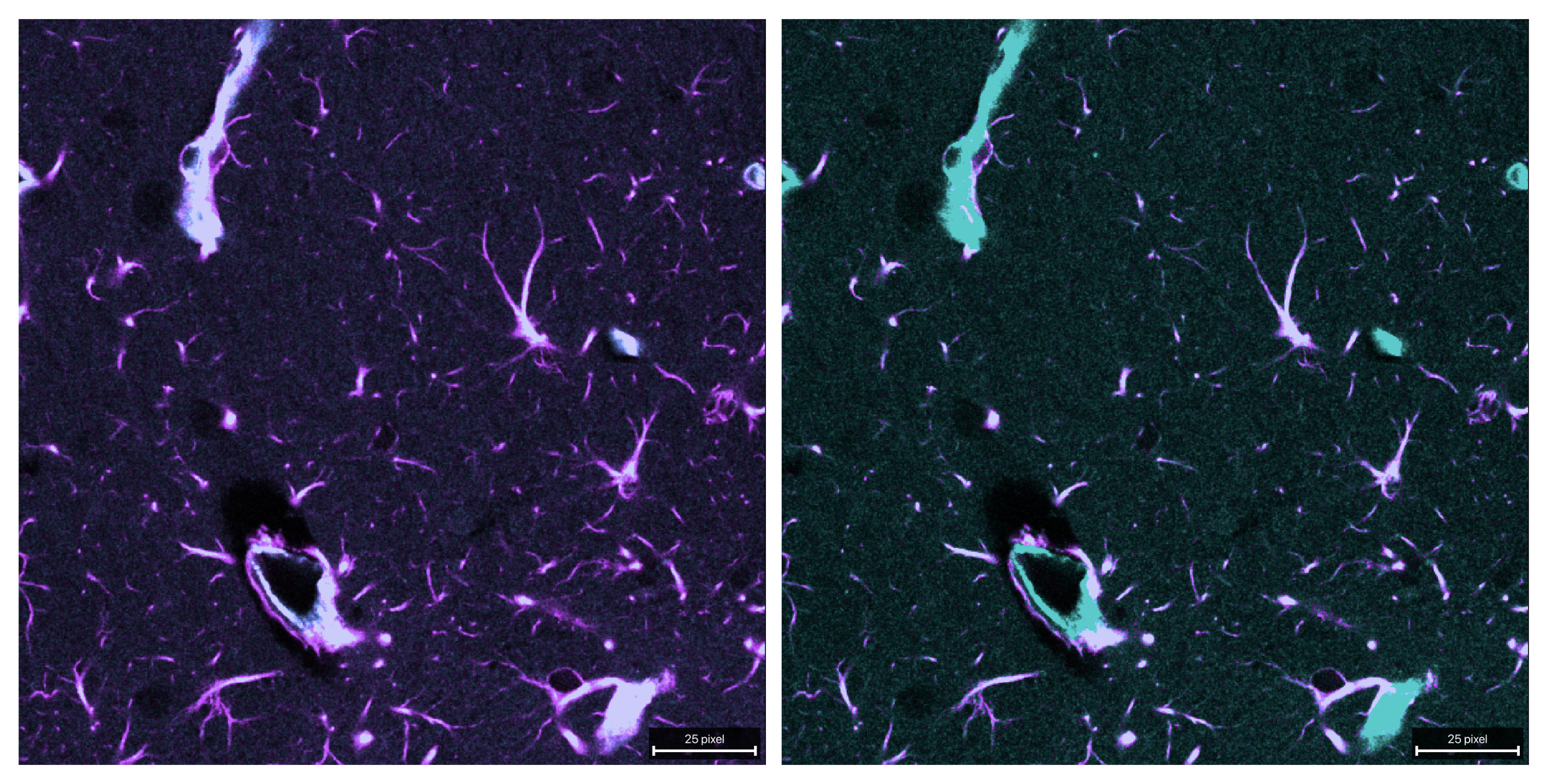
Both channels after unmixing with the mean-ratio method. The bleed-through from channel 0 into channel 1 is largely removed, while the original signal in channel 1 is preserved. Note that the estimated alpha is slightly different from the fixed value of 0.62 used in the previous example, as it is computed from the data itself. Thus, the resulting unmixed image slightly differs in the quality of bleed-through removal and the preservation of the original signal in channel 1.

Composite comparison of the raw (left) and unmixed (right) stack.

linear_fit method

This variant estimates alpha via masked least squares without an intercept. Use this when you want a fit-based coefficient rather than the simpler ratio of means. It relies on the same mask and preprocessing parameters as the mean_ratio method:

OUTPUT_REFERENCE_LINEAR_FIT = OUTPUT_DIR / f"{INPUT_NAME}_unmixed_reference_t0_linear_fit.tif"

reference_linear_fit_output = unmix(
    input_path=INPUT_PATH,
    output_path=OUTPUT_REFERENCE_LINEAR_FIT,
    # source_channel=0,  # default: 0
    # target_channel=1,  # default: 1
    # alpha_mode="reference_t",
    # alpha_reference_t=0,
    method="linear_fit",
    signal_percentile=99.0,
    background_percentile=1.0,
    # target_low_percentile=95.0,
    # preprocess_alpha_inputs=True,  # default: True
    # clip_negative=True,  # default: True
)
print(reference_linear_fit_output)
print(report_path_from_output_path(reference_linear_fit_output).read_text(encoding="utf-8"))
show_unmixed_channels_in_napari(
    reference_linear_fit_output,
    source_channel=0,
    target_channel=1,
    layer_prefix="Reference linear_fit")

Useful optional controls are the same as for mean_ratio:

• target_low_percentile

• preprocess_alpha_inputs

• clip_negative

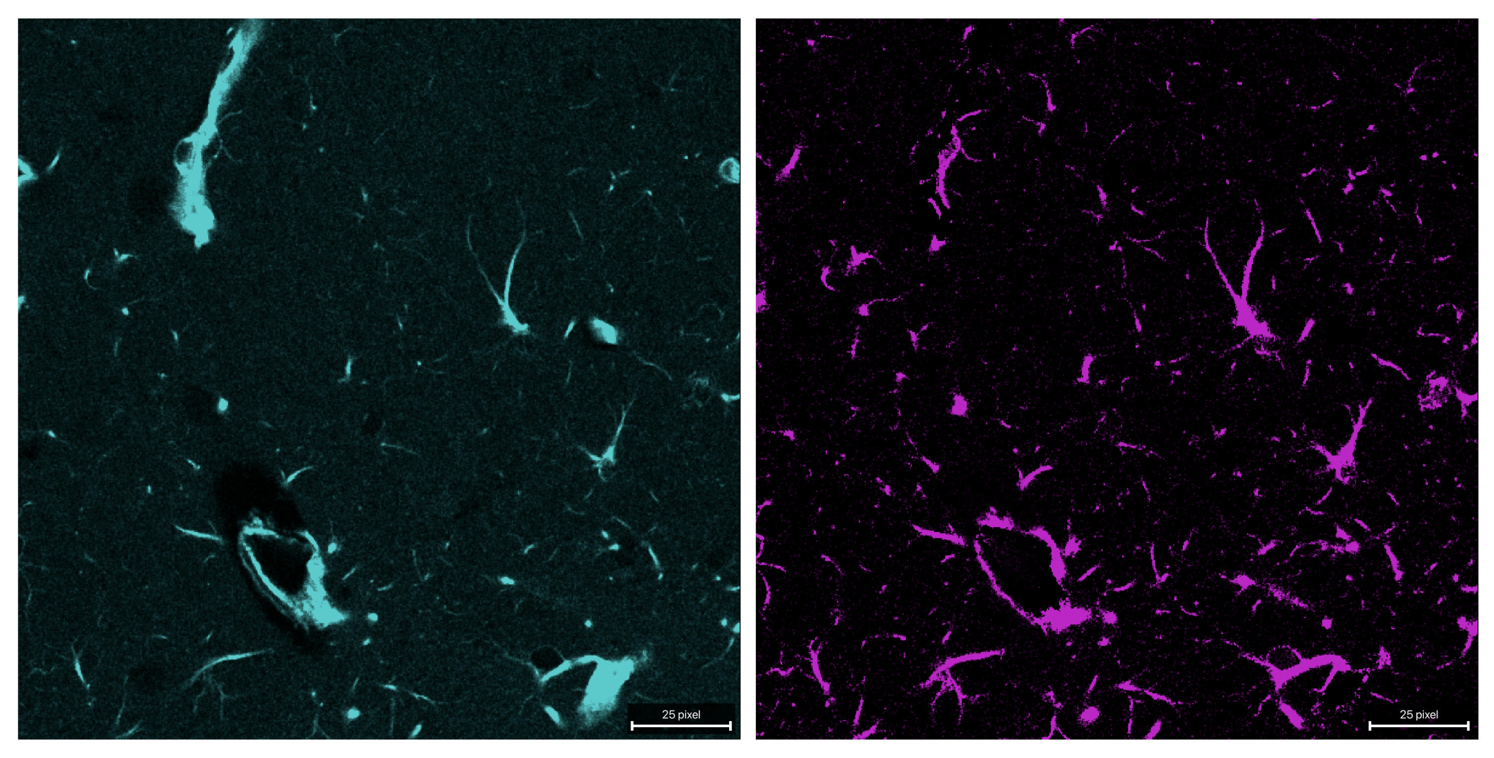
Both channels after unmixing with the linear-fit method. Here, alpha is estimated via masked least squares, which can provide a more robust estimate in the presence of noise or outliers compared to the mean-ratio method. The bleed-through from channel 0 into channel 1 is effectively removed, while the original signal in channel 1 is preserved.

Composite comparison of the raw (left) and unmixed (right) stack.

corr_min method

This method chooses alpha such that correlation between the source channel and the corrected target channel is minimized.

Useful parameters include:

• alpha_max: upper bound of the optimization interval

• the same mask-related parameters as above

This method can be more aggressive than simple ratio-based estimation when source and target channels are biologically correlated:

OUTPUT_REFERENCE_CORR_MIN = OUTPUT_DIR / f"{INPUT_NAME}_unmixed_reference_t0_corr_min.tif"

reference_corr_min_output = unmix(
    input_path=INPUT_PATH,
    output_path=OUTPUT_REFERENCE_CORR_MIN,
    # source_channel=0,  # default: 0
    # target_channel=1,  # default: 1
    # alpha_mode="reference_t",
    # alpha_reference_t=0,
    method="corr_min",
    signal_percentile=99.0,
    background_percentile=1.0,
    alpha_max=1.0,
    # target_low_percentile=95.0,
    # preprocess_alpha_inputs=True,  # default: True
    # max_alpha_voxels=500_000,  # default
    # random_state=0,  # default
)
print(reference_corr_min_output)
print(report_path_from_output_path(reference_corr_min_output).read_text(encoding="utf-8"))
show_unmixed_channels_in_napari(
    reference_corr_min_output,
    source_channel=0,
    target_channel=1,
    layer_prefix="Reference corr_min")

Additional optional controls worth knowing are:

• target_low_percentile

• preprocess_alpha_inputs

• max_alpha_voxels

• random_state

Both channels after unmixing with the corr-min method. Here, alpha is estimated via correlation minimization, which can be particularly effective when the source and target channels are biologically correlated.

Composite comparison of the raw (left) and unmixed (right) stack.

mi_min method

This method uses a PICASSO-like criterion in the two-channel case by choosing alpha to minimize mutual information between the source channel and the corrected target channel.

Important user-tunable parameters:

• mi_bins: histogram resolution for the mutual-information estimate. Higher values can resolve finer structure but also become noisier; lower values are coarser and usually more stable.

• alpha_max: upper search bound for the optimized alpha. Larger values allow stronger subtraction; smaller values constrain the optimizer more conservatively.

• mask and background settings

OUTPUT_REFERENCE_MI_MIN = OUTPUT_DIR / f"{INPUT_NAME}_unmixed_reference_t0_mi_min.tif"

reference_mi_min_output = unmix(
    input_path=INPUT_PATH,
    output_path=OUTPUT_REFERENCE_MI_MIN,
    # source_channel=0,  # default: 0
    # target_channel=1,  # default: 1
    # alpha_mode="reference_t",
    # alpha_reference_t=0,
    method="mi_min",
    signal_percentile=50.0,
    background_percentile=1.0,
    alpha_max=1.0,
    mi_bins=64,
    # target_low_percentile=95.0,
    # preprocess_alpha_inputs=True,  # default: True
    # max_alpha_voxels=500_000,  # default
    # random_state=0,  # default
)
print(reference_mi_min_output)
print(report_path_from_output_path(reference_mi_min_output).read_text(encoding="utf-8"))
show_unmixed_channels_in_napari(
    reference_mi_min_output,
    source_channel=0,
    target_channel=1,
    layer_prefix="Reference mi_min")

Further optional controls are:

• target_low_percentile

• preprocess_alpha_inputs

• max_alpha_voxels

• random_state

Both channels after unmixing with the mi-min method. Here, alpha is estimated via mutual information minimization, which can be particularly effective when the source and target channels are biologically correlated.

Composite comparison of the raw (left) and unmixed (right) stack.

What to change for your own data

For a new dataset, the main things to adapt are:

• INPUT_PATH

• source_channel and target_channel

• your chosen alpha strategy: fixed, reference-time-point, or another method

• mask strictness via signal_percentile and target_low_percentile

If a reliable single-label control exists, start with the fixed-alpha mode first. It usually gives the most interpretable baseline.