Filtering, registration, and projection helper example
Unlike the unmixing tutorials, this page focuses on the optional helper
functions that are useful after spectral unmixing has already been performed.
The script demonstrates a practical post-processing workflow for a canonical
TZCYX stack:
loading the stack with OMIO,
correcting intra-stack z-drift,
registering the stack across time,
matching intensities across time,
filtering before and after projection,
projecting along z,
and saving the final processed result.
How to use this tutorial
All steps described in this tutorial are implemented in the Python script
user_scripts/filter_and_register_stack.py. The script is designed
for interactive execution in a cell-based editor such as
VS Code’s interactive window.
The recommended workflow is:
open
user_scripts/filter_and_register_stack.py,run the cells from top to bottom,
adapt the settings that are relevant for your own dataset.
The subsections below follow the order of the script cells and explain what the individual helper functions are doing and which settings matter most.
The script and this tutorial mimic a typical post-processing workflow for a time-lapse z-stack, but you can also use the individual helper functions in a different order or with different settings if your own dataset requires it. The main takeaway point is, that you can combine the package’s non-unmixing modules in a flexible way to build your own post-processing pipeline, tailored to your own data and analysis needs.
What this tutorial covers
This helper workflow demonstrates how the package’s non-unmixing modules can be combined in a realistic pipeline:
OMIO-based stack loading and saving,
within-time-point z-drift correction via
correct_intra_stack_z_drift(...),across-time registration via
register_stack(...),time-wise intensity harmonization via
match_histograms_across_time(...),filtering via
apply_filters(...),and z-projection via
max_z_project(...).
This makes the tutorial a good starting point when you already have an unmixed stack and want to continue with structural cleanup and visualization-oriented processing.
Imports
The first cell imports the package helpers used throughout the tutorial:
from __future__ import annotations

from pathlib import Path

PROJECT_ROOT = Path(__file__).resolve().parents[1]

from spectral_unmixing.io import load_stack_with_omio, write_stack_with_omio
from spectral_unmixing.registration import correct_intra_stack_z_drift, register_stack
from spectral_unmixing.filters import (
    apply_filters,
    match_histograms_across_time,
    max_z_project)

import omio as om
The most important imported functions here are:
load_stack_with_omio(...)andwrite_stack_with_omio(...)for I/O,correct_intra_stack_z_drift(...)andregister_stack(...)for registration,apply_filters(...),match_histograms_across_time(...), andmax_z_project(...)for post-processing.
Define input and output paths
Next, we need to define the input stack and the output directory where the processed result will be written:
INPUT_PATH = (PROJECT_ROOT / "example_data" / "Gockel_Nieves_Rivera_2026" / "Gockel_Nieves_Rivera_2026_5D_stack.tif")
INPUT_NAME = INPUT_PATH.stem

OUTPUT_DIR = INPUT_PATH.parent / "registered"
OUTPUT_DIR.mkdir(parents=True, exist_ok=True)
OUTPUT_PATH = OUTPUT_DIR / f"{INPUT_NAME}_registered.tif"
What you will usually change here:
INPUT_PATHto point to your own OMIO-readable stack,the output directory name,
and the output filename pattern.
Load the stack
The next cell loads the input stack and prints a quick shape and axis summary:
stack, metadata = load_stack_with_omio(INPUT_PATH)
print(f"Loaded stack: {stack.shape}, axes={metadata.get('axes')}")
# %% INSPECT STACK IN NAPARI
om.open_in_napari(stack, metadata, "Unregistered |")
This is a good early sanity check. Before any processing is applied, confirm
that the stack shape is what you expect and that the metadata report canonical
TZCYX axes.
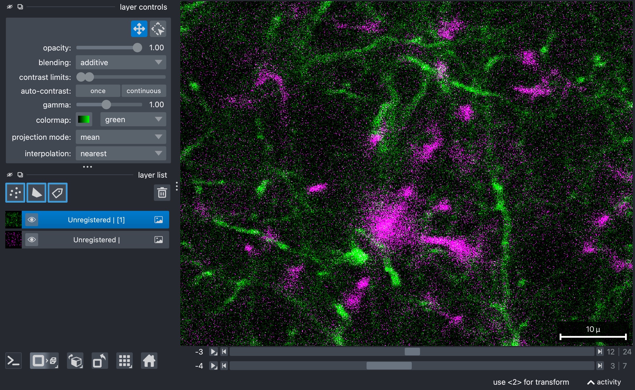
Raw two-channel example stack (3D+t) used in this tutorial. Shown is slice z=12 at t=3.
Correct intra-stack z-drift
This cell uses correct_intra_stack_z_drift(...) to compensate for z-local
motion within each time point before any across-time registration is attempted:
z_corrected_stack = correct_intra_stack_z_drift(
    stack,
    registration_channel=0,  # can also be 1 if channel 1 is the more stable structure
    method="pystackreg",  # "phase_cross_correlation" "pystackreg"
    reference_mode="neighbor",  # or "full_projection"
    neighbor_window_size=3,  # 3 -> z-1, z, z+1; 5 -> z-2 ... z+2
    pre_median_filter=True,
    post_median_filter=False,
    median_kernel_size=3,
    verbose=True)

print(f"Z-corrected stack: {z_corrected_stack.shape}")
z_corrected_metadata = om.update_metadata_from_image(metadata, z_corrected_stack)
om.open_in_napari(stack, metadata, "Unregistered |")
om.open_in_napari(z_corrected_stack, z_corrected_metadata, "Z-corrected |")
The most important settings here are:
registration_channel: chooses which channel is treated as the structurally stable reference for z-drift correction. Pick the channel that contains the most reliable non-motile structure.method: selects the registration backend; currently supported are"pystackreg"and"phase_cross_correlation".reference_mode: determines how each z-slice is compared."neighbor"uses a local neighboring-slice reference, whereas other modes such as"full_projection"can be more global and aggressive.neighbor_window_size: controls how many neighboring z-slices participate in the local reference whenreference_mode="neighbor". Larger values make the local reference broader; smaller values keep it more local.pre_median_filterandpost_median_filter: control whether median filtering is applied before or after generating the registration reference images. Note: Removing noise can improve registration, depending on the dataset. Filtering is applied only ti the internal reference images, not to the original stack nor the final output.median_kernel_size: sets the kernel size for those optional median filters.verbose: enables terminal output during the correction run.
The napari calls in this cell are useful for visually comparing the original and z-corrected stacks before continuing.
:: note
Since the underlying example stack is already well-aligned in z, we omitted this step here. The same is true for the subsequently discussed registration across time. In practice, you will usually want to run movement corrections before any further processing, since even small misalignments can affect downstream interpretation and analysis.
Register the stack across time
Once intra-stack z-drift has been reduced, you can additionally register the corrected stack across time:
registered_stack = register_stack(
    z_corrected_stack,
    registration_channel=0,
    method="pystackreg", # phase_cross_correlation or pystackreg
    zrange=None,
    pre_median_filter=True,
    post_median_filter=True,
    median_kernel_size=5)
print(f"Registered stack: {registered_stack.shape}")
registered_metadata = om.update_metadata_from_image(metadata, registered_stack)
om.open_in_napari(registered_stack, registered_metadata, "Registered |")
The most relevant settings are:
registration_channel: same role as above, but now for across-time registration.method: again selects the registration backend.zrange: limits which z-slices are included in the projection used to estimate the time-registration shifts. This can help when only part of the z-stack contains the stable structure you want to align on.pre_median_filterandpost_median_filter: optional denoising applied before and after building the registration reference images.median_kernel_size: kernel size for those optional median filters.
This step estimates one spatial shift per time point and applies the result to the original 3D stack, not only to the projected reference images. The latter only serve to compute the shifts, but the full 3D+t stack is shifted accordingly.
Match histograms across time
After geometry has been aligned, one can use the script to harmonize the intensity distributions across time:
# Recommendation: do this after registration and before Z projection so that
# geometry is already aligned, but the full 3D time stacks are still available.
matched_registered_stack = match_histograms_across_time(registered_stack, reference_t=0)
print(f"Histogram matched stack: {matched_registered_stack.shape}")
matched_registered_metadata = om.update_metadata_from_image(metadata, matched_registered_stack)
om.open_in_napari(matched_registered_stack, matched_registered_metadata, "Registered + hist matched |")
The key setting is:
reference_t: defines which time point serves as the intensity reference. The remaining time points are histogram-matched to that stack.
This is useful when slow brightness drift would otherwise make later comparisons or visualizations harder to interpret.
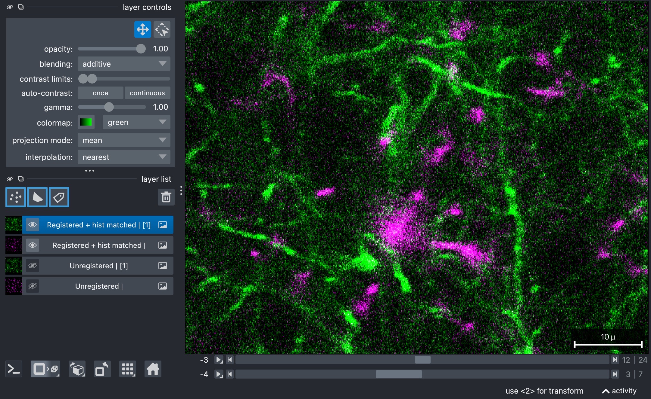
Histogram-matched two-channel example stack (3D+t). Histogram matching is useful when slow brightness drift would otherwise make later comparisons or visualizations harder to interpret. Shown is slice z=12 at t=3.
Filter the registered stack
The next step includes applying a simple filter chain to the full registered stack:
filtered_stack = apply_filters(
    matched_registered_stack,
    filters=["median", "gaussian"],
    median_size=3,
    gaussian_sigma=1.0,
    apply_3d=False)
print(f"Filtered stack: {filtered_stack.shape}")
filtered_metadata = om.update_metadata_from_image(metadata, filtered_stack)
om.open_in_napari(filtered_stack, filtered_metadata, "Filtered |")
The main settings are:
filters=["median", "gaussian"]: defines the ordered filter sequence. The filters are applied in exactly this order.median_size: kernel size of the median filter.gaussian_sigma: smoothing strength of the Gaussian filter.apply_3d: controls whether filtering is applied slice-wise in 2D or volumetrically in 3D. Here it is kept atFalse, so each z-slice is filtered individually.
This stage is often useful for reducing noise slice-wise for each time point, in order to improve downstream visualization or analysis.
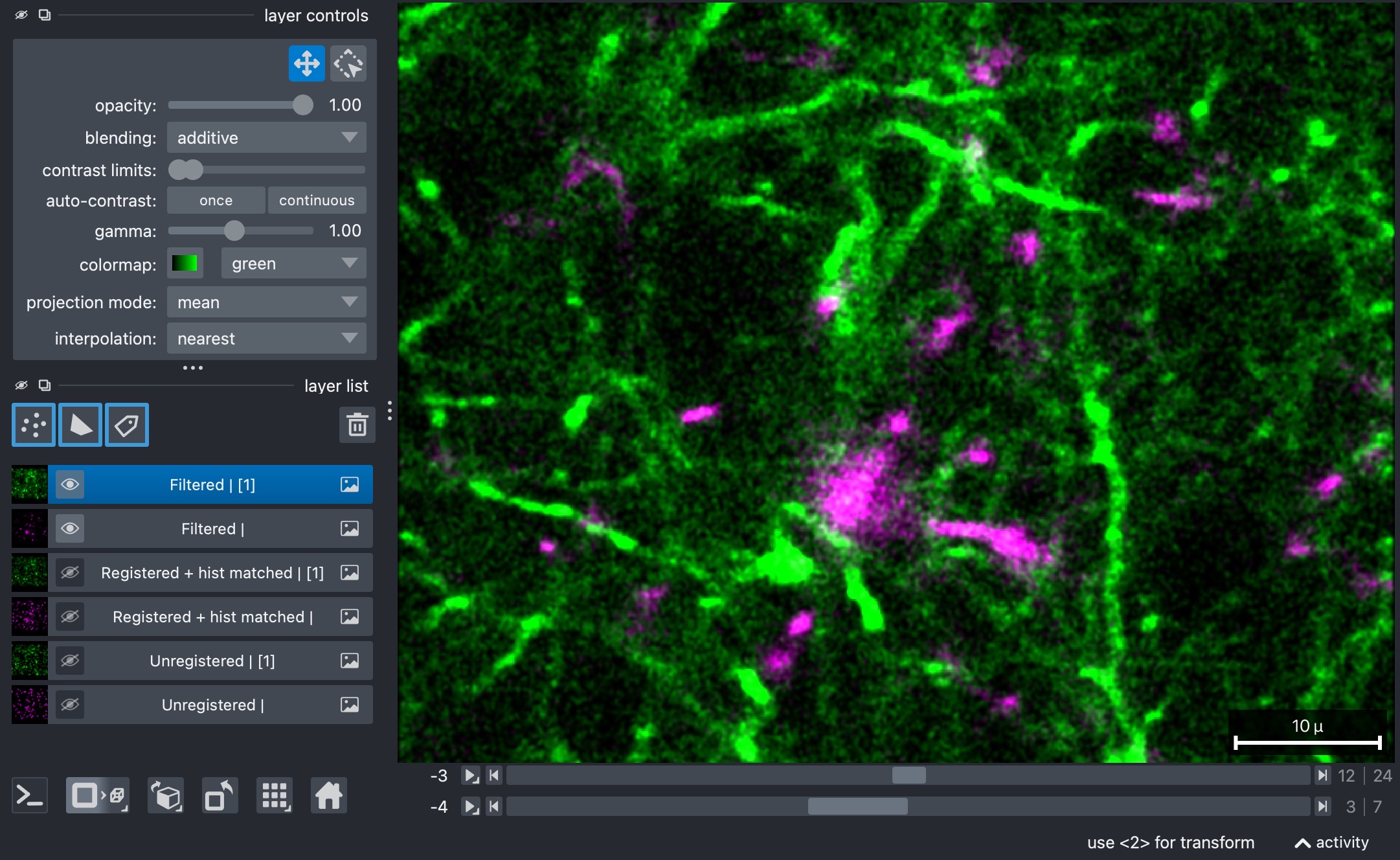
Histogram-matched two-channel example stack (3D+t) after slice-wise 2D filtering. Filtering is often useful for reducing noise slice-wise for each time point, in order to improve downstream visualization or analysis. Shown is slice z=12 at t=3.
Project along z
For visualization purposes or for subsequent 2D analysis, it is often useful to project
the 3D+t stack along z. Our helper function max_z_project(...) computes a maximum-intensity
projection along the z-axis over a selected z-range:
zrange=(0,10) # None or (start_z, end_z) to specify a range of z-slices to project.
            # If None, the full z-range is projected.
projected_stack = max_z_project(filtered_stack, zrange=zrange)
print(f"Projected stack: {projected_stack.shape}")
projected_metadata = om.update_metadata_from_image(metadata, projected_stack)
# temp_projected_path = OUTPUT_DIR / "ID14135_TP0_d2_unmixed_fixed_alpha_registered_histmatched_projected_tmp.tif"
# temp_projected_saved = write_stack_with_omio(temp_projected_path, projected_stack, metadata)
om.open_in_napari(projected_stack, projected_metadata, "Projected |")
The key setting is:
zrange: eitherNonefor the full z-stack or a tuple(start_z, end_z)for a restricted projection range.
Restricting the z-range can be useful when only part of the stack contains the structures of interest and the remaining slices would mainly add blur or background.
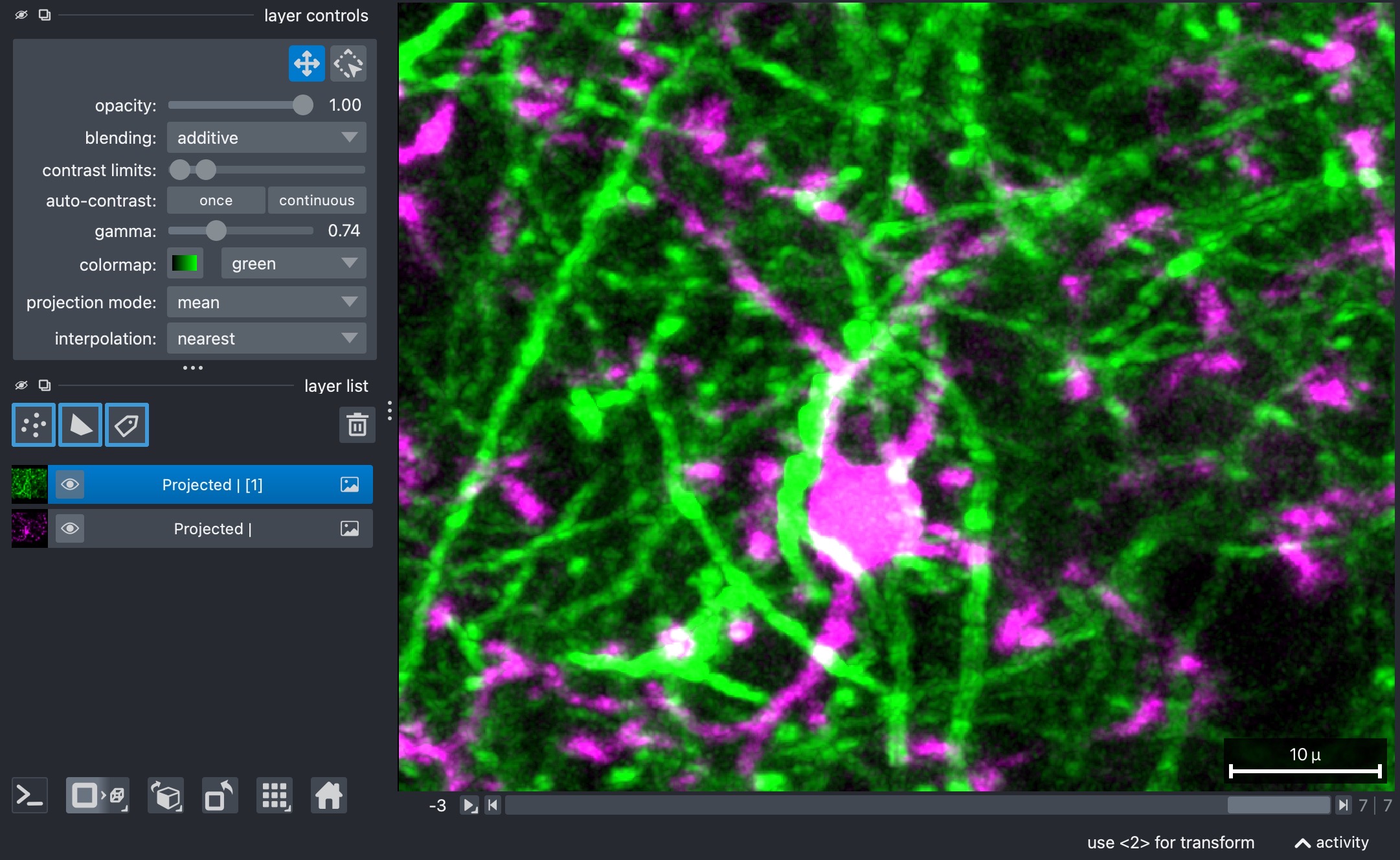
2D maximum-intensity projection of the histogram-matched two-channel example stack (3D+t) after slice-wise 2D filtering. The projection is computed along the z-axis over a cropped z-range. Restricting the z-range can be useful when only part of the stack contains the structures of interest and the remaining slices would mainly add blur or background.
Filter the projected stack again
After projection, you can apply another filter chain to the now 2D+t result:
filtered_projected_stack = apply_filters(
    projected_stack,
    filters=["median", "gaussian"],
    median_size=3,
    gaussian_sigma=1.5,
    apply_3d=False)
print(f"Filtered projected stack: {filtered_projected_stack.shape}")
filtered_projected_metadata = om.update_metadata_from_image(metadata, filtered_projected_stack)
om.open_in_napari(filtered_projected_stack, filtered_projected_metadata, "Filtered Projected |")
The same filter logic is used as before, but the post-projection settings can be tuned separately. This is often helpful because a projected image may benefit from slightly stronger smoothing than the original 3D stack.
Here, the most important adjustable parameters are again:
filtersmedian_sizegaussian_sigmaapply_3d: still kept atFalsebecause the projected stack is already effectively two-dimensional along z.
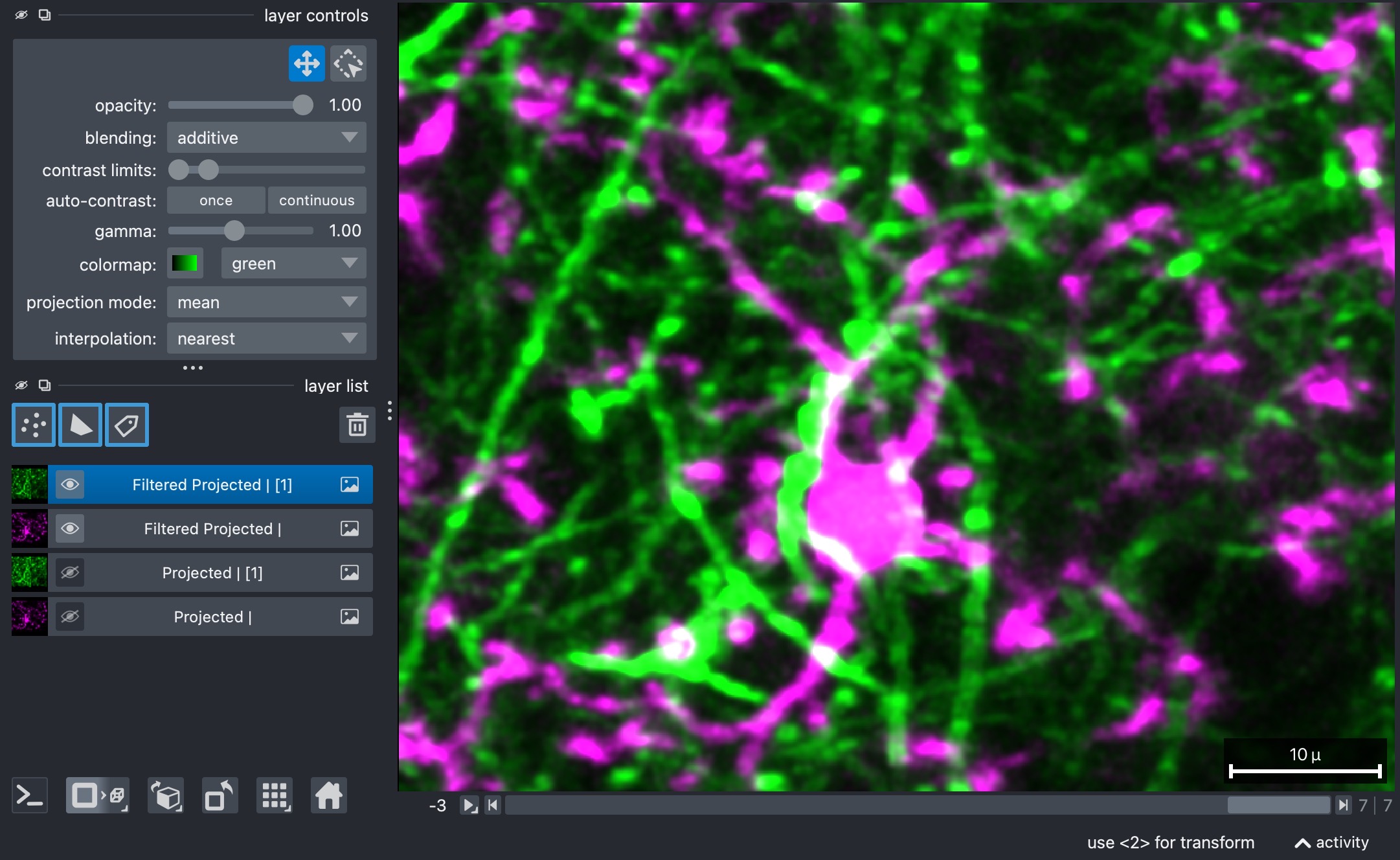
Final 2D+t result after post-projection filtering of the maximum-intensity projection of the histogram-matched two-channel example stack (3D+t). Filtering the projected stack again can be useful because a projected image may benefit from slightly stronger smoothing than the original 3D stack.
Save the processed stack
When you are done, you can save the processed projected stack back to disk:
filtered_projected_path = OUTPUT_DIR / f"{INPUT_NAME}_registered_histmatched_filtered_projected_z{zrange[0]}_to_{zrange[1]}.tif"
filtered_projected_saved = write_stack_with_omio(filtered_projected_path, filtered_projected_stack, metadata)
Fine-tuning
The script shown in this tutorial uses a straightforward helper workflow with
one shared filter configuration before projection and another one after
projection. In practice, some datasets need more selective tuning.
For that, have a look at
user_scripts/fine_filter_and_register_stack.py. We do not provide a
separate step-by-step tutorial page for it, but it demonstrates the next level
of control:
separate filter chains for the second channel via
filters_channel2,channel-specific overrides such as
median_size_channel2andgaussian_sigma_channel2,per-time-point filter strengths by passing lists for
median_sizeorgaussian_sigma, andseparate post-projection filter settings.
If the basic helper script works but one channel is still too noisy or one time point clearly needs stronger or weaker filtering than the others, that fine-tuning script is the right next place to continue.