Full 3D+t unmixing example

This tutorial documents the interactive script user_scripts/unmix_full_TZCYX_synthetic_example.py. It extends the basic two-channel workflow to a full canonical TZCYX stack with multiple time points and multiple z-slices.

How to use this tutorial

The script is meant to be run as an interactive Python script in an editor that supports cell-based execution.

The recommended workflow is:

1. open user_scripts/unmix_full_TZCYX_synthetic_example.py,

2. run the cells from top to bottom,

3. adapt the parameters that matter for your own data.

The subsections below follow the same order as the script.

What this tutorial covers

Compared with Basic unmixing example, this script adds three important practical ingredients:

• a full T > 1 and Z > 1 stack,

• a synthetic dataset with known bleed-through,

• and a per-time-point alpha-estimation example.

That makes it a good bridge between the simplest public example and a real time-lapse z-stack workflow.

Imports

The imported helpers are the same as in the simpler two-channel tutorial:

• unmix(...) for the actual spectral unmixing,

• report_path_from_output_path(...) for inspecting the JSON sidecar,

• show_unmixed_channels_in_napari(...) for visual inspection.

Define input and output paths

INPUT_PATH = PROJECT_ROOT / "example_data" / "synthetic_data" / "synthetic_bleedthrough_T9_Z20_C2.tif"
INPUT_NAME = INPUT_PATH.stem
OUTPUT_DIR = INPUT_PATH.parent / "unmixed"
OUTPUT_DIR.mkdir(parents=True, exist_ok=True)
# %% OPTIONAL: INSPECT PREPARED STACKS IN NAPARI
from spectral_unmixing.viewer import show_all_channels_in_napari
show_all_channels_in_napari(INPUT_PATH, layer_prefix="3D+t synthetic simulation")

What you would usually change here:

• INPUT_PATH to your own OMIO-readable stack,

• the output directory or filename pattern.

Manually set alpha

OUTPUT_FIXED = OUTPUT_DIR / f"{INPUT_NAME}_unmixed_fixed_alpha.tif"

fixed_output = unmix(
    input_path=INPUT_PATH,
    output_path=OUTPUT_FIXED,
    # source_channel=0,  # default: 0
    # target_channel=1,  # default: 1
    alpha=0.62,
    alpha_mode="fixed",
    method="manual",
    # clip_negative=True,  # default: True
    # output_dtype="float32",  # default: "float32"
    # verbose=True,  # default: True
)

show_unmixed_channels_in_napari(
    fixed_output,
    source_channel=0,
    target_channel=1,
    layer_prefix="Fixed alpha",
    source_colormap="cyan",
    target_colormap="yellow")

This is the simplest baseline on the full stack. The exact same fixed alpha is applied across all time points and all z-slices.

The most relevant parameters are:

• method="manual": uses the user-provided alpha directly instead of estimating it from the data.

• alpha: sets the subtraction strength. Larger values remove more source contribution; smaller values leave more residual bleed-through.

• alpha_mode: can be set explicitly to fixed, but this is not required. The default is None. When alpha_mode=None and a user-provided alpha is present, the pipeline internally resolves to fixed.

• optional source_channel and target_channel: define the direction of correction through the full TZCYX stack.

• optional clip_negative: clips negative corrected intensities to zero after subtraction.

This is the best starting point when you already have a coefficient from a proper control measurement or an empirical estimate from a similar dataset.

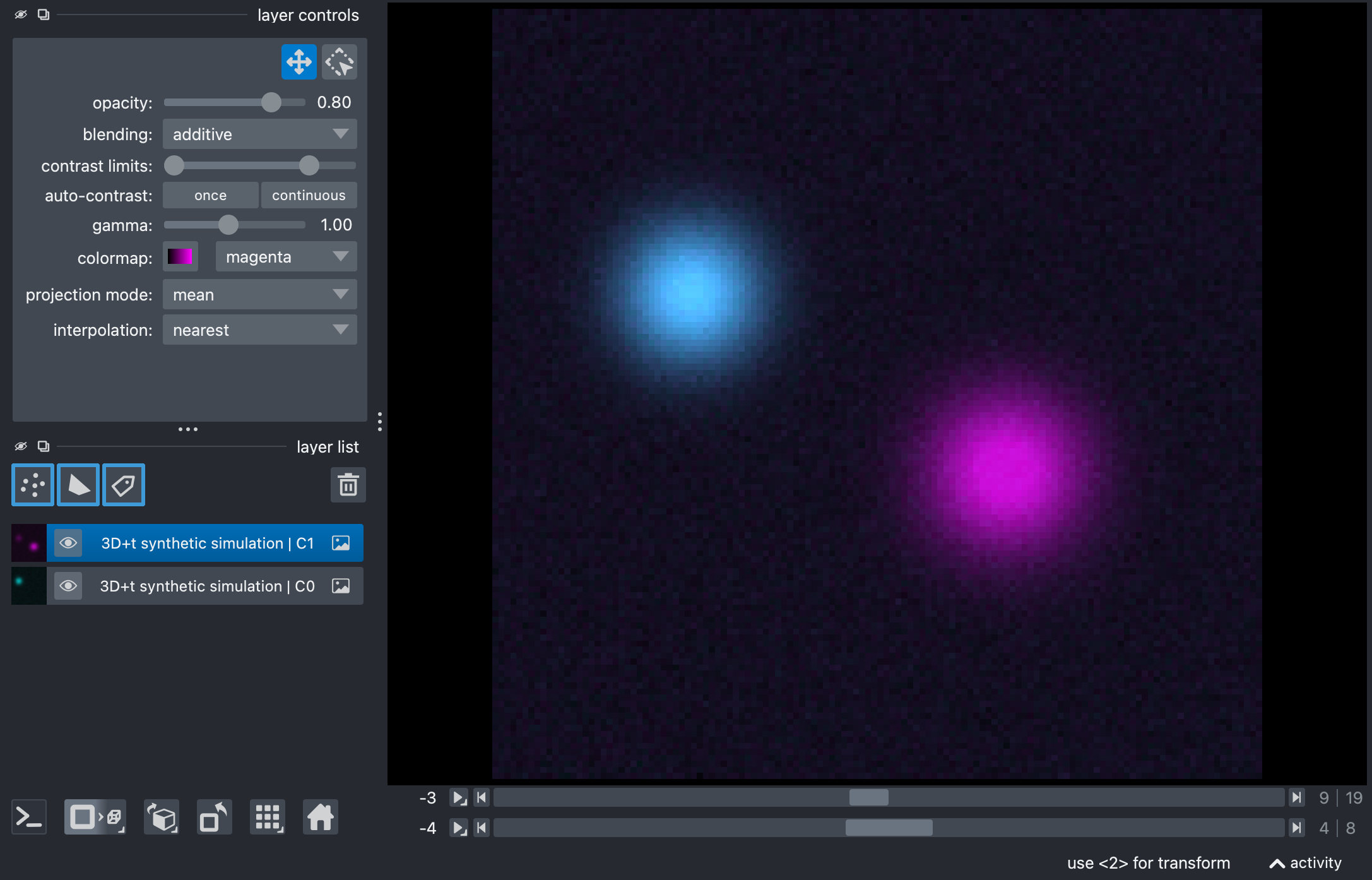
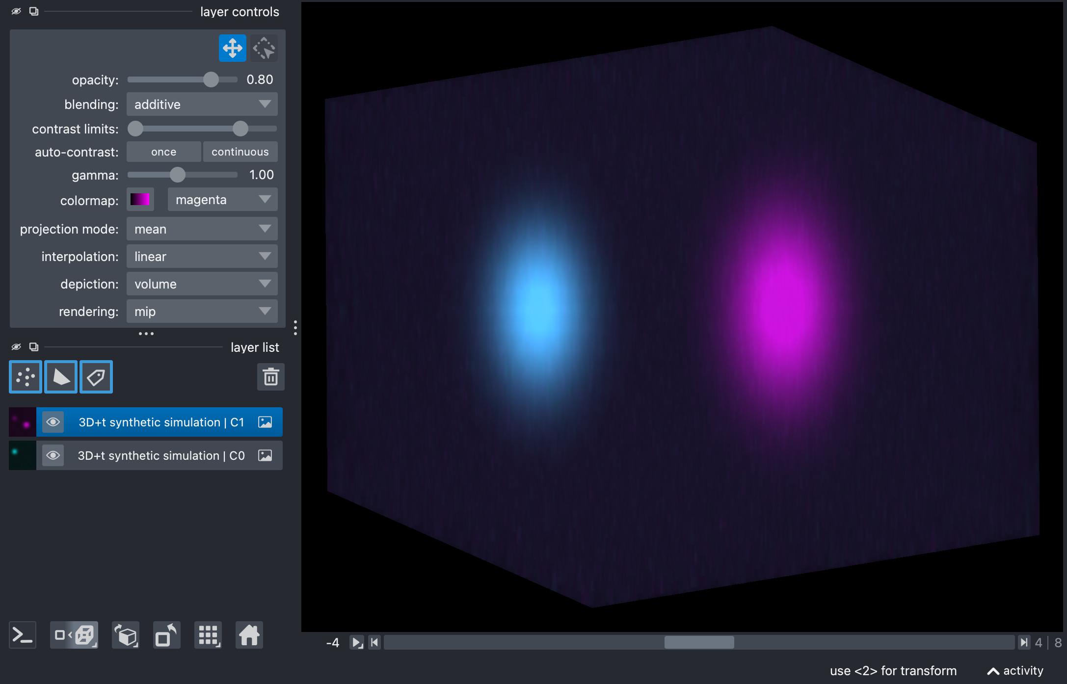
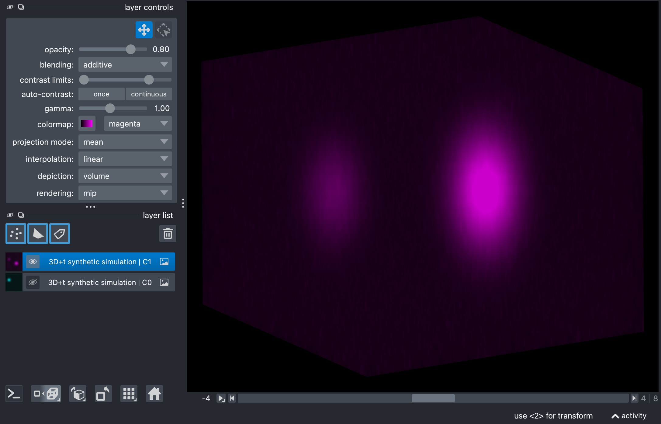
Composite images of the raw synthetic stack, showing the source and target channels in Napari’s 2D (top) and 3D views (center). The source channel is shown in cyan, and the target channel is shown in magenta. The images illustrate the bleed-through from the source to the target channel (bottom), which will be corrected by the unmixing process.

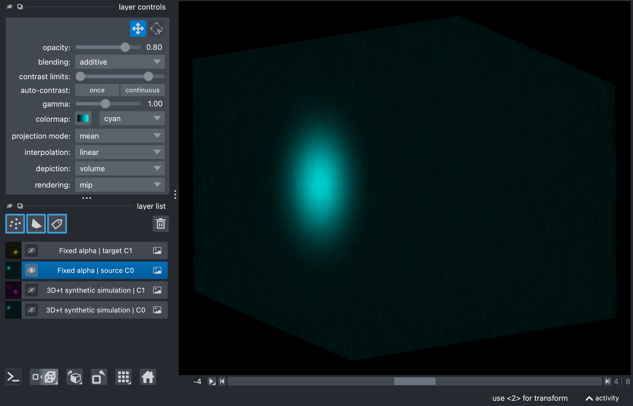
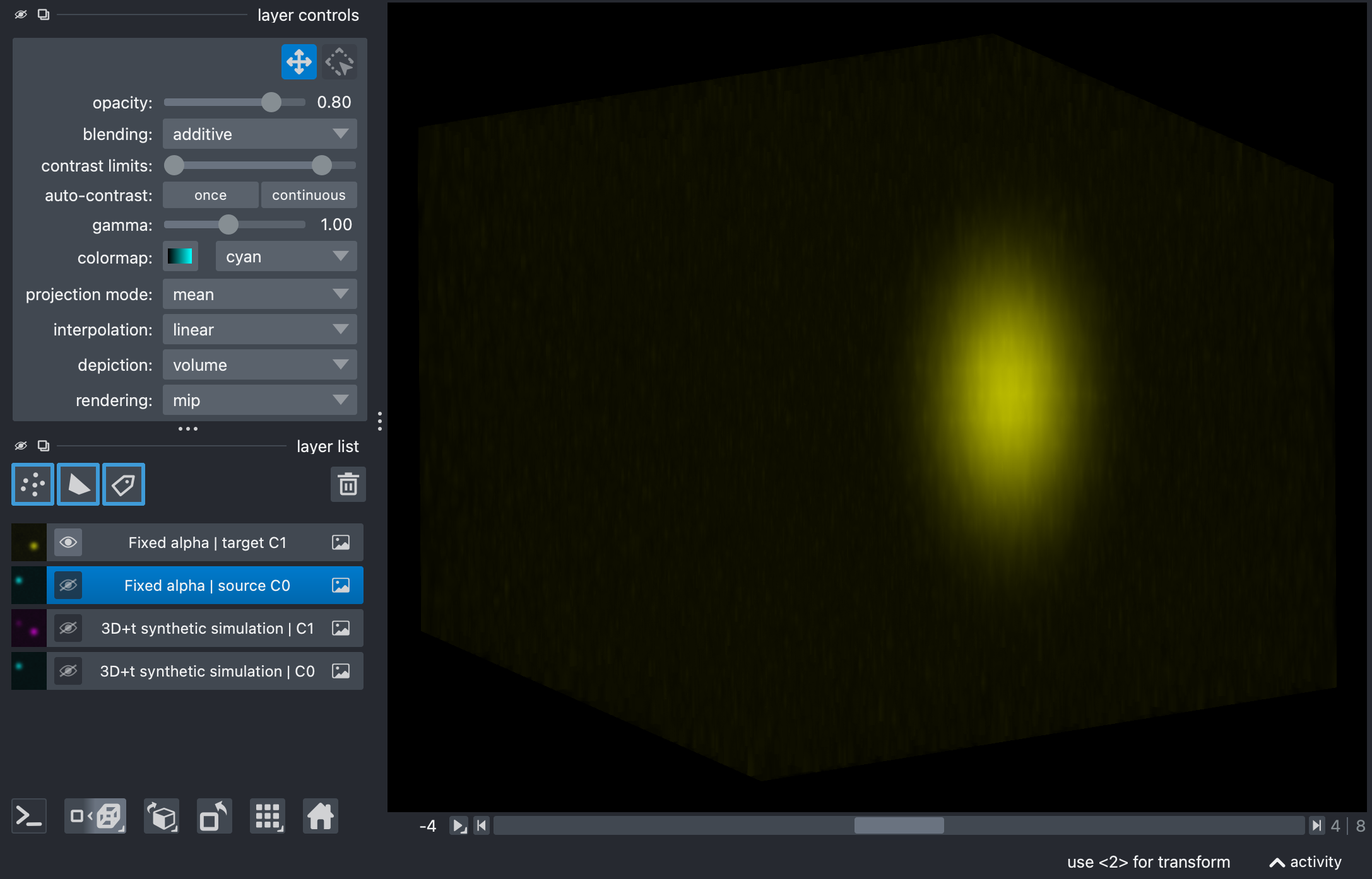
Results of the fixed-alpha unmixing on the synthetic stack, showing the source (top) and target (bottom) channels in Napari’s 3D view. The bleed-through from the source to the target channel has been corrected. The subsequent examples show how to estimate alpha automatically from the data, always resulting in a similar final output (and therefore omitted here for brevity).

mean_ratio on a full TZCYX stack

OUTPUT_REFERENCE = OUTPUT_DIR / f"{INPUT_NAME}_unmixed_reference_t0_mean_ratio.tif"

reference_output = unmix(
    input_path=INPUT_PATH,
    output_path=OUTPUT_REFERENCE,
    # source_channel=0,  # default: 0
    # target_channel=1,  # default: 1
    alpha_mode="reference_t",
    # alpha_mode="per_t",  # use the same estimator separately at each time point
    method="mean_ratio",
    alpha_reference_t=0, # only relevant for alpha_mode="reference_t"
    signal_percentile=50.5,
    target_low_percentile=96.0,
    background_percentile=0.5,
    preprocess_alpha_inputs=False,
    clip_negative=True,
)
print(reference_output)
print(report_path_from_output_path(reference_output).read_text(encoding="utf-8"))
show_unmixed_channels_in_napari(
    reference_output,
    source_channel=0,
    target_channel=1,
    layer_prefix="Reference t0")

This is the simplest automatic estimator on a given dataset. It computes the ratio of mean intensities inside a bright-source mask.

If alpha_mode is left unset or explicitly set to None, the pipeline does not stay in a hidden fixed mode. Instead, because no manual alpha is provided here and method!="manual", the workflow automatically falls back to alpha_mode="reference_t" with alpha_reference_t=0. That default works for both T=1 and T>1 stacks.

In this script the method is demonstrated explicitly with alpha_mode="reference_t", where one alpha is estimated from the selected reference time point, using all z-slices belonging to that time point, and then applied to all time points. The same mean_ratio estimator can also be combined with alpha_mode="per_t" when you want one separately estimated coefficient per time point.

The parameters that matter most are:

• alpha_mode: reference_t or per_t. The former estimates one alpha from the reference time point; the latter estimates one alpha per time point. If this argument is omitted or set to None, the pipeline defaults to reference_t with alpha_reference_t=0 for non-manual methods such as the present mean_ratio example.

• alpha_reference_t: defines the reference time point used for alpha estimation using alpha_mode="reference_t". Changing it matters when the stack changes in brightness, content, or other properties such as SNR over time.

• signal_percentile: defines how selective the bright-source mask is. Higher values keep only the brightest source voxels; lower values include more voxels and therefore more mixed regions.

• background_percentile: defines the low-intensity background estimate subtracted before alpha estimation. Higher values remove more baseline; lower values preserve more of the dim signal.

• target_low_percentile: can further restrict the estimation mask to target-dim voxels. Lower values make that restriction stricter, higher values relax it.

• preprocess_alpha_inputs: controls whether the percentile-based preprocessing is applied before estimating alpha. Turning it off makes the estimate more directly dependent on the raw stack intensities.

Note

If you explicitly set alpha_mode="reference_t" on a stack that effectively has only one time point (T=1), the pipeline simply uses t=0 as the only valid reference time point. If you explicitly set alpha_mode="per_t" on a T=1 stack, the pipeline does not fail either: it just estimates one alpha value for that single time point. In other words, both modes remain valid for T=1 data; they just collapse to the only available time index.

linear_fit on a full TZCYX stack

OUTPUT_REFERENCE_LINEAR_FIT = OUTPUT_DIR / f"{INPUT_NAME}_unmixed_reference_t0_linear_fit.tif"

reference_linear_fit_output = unmix(
    input_path=INPUT_PATH,
    output_path=OUTPUT_REFERENCE_LINEAR_FIT,
    # source_channel=0,  # default: 0
    # target_channel=1,  # default: 1
    alpha_mode="reference_t",
    # alpha_mode="per_t",  # same estimator, but one fitted alpha per time point
    method="linear_fit",
    alpha_reference_t=0,
    signal_percentile=99.0,
    background_percentile=1.0,
    # target_low_percentile=95.0,
    # preprocess_alpha_inputs=True,  # default: True
    # clip_negative=True,  # default: True
)
print(reference_linear_fit_output)
print(report_path_from_output_path(reference_linear_fit_output).read_text(encoding="utf-8"))
show_unmixed_channels_in_napari(
    reference_linear_fit_output,
    source_channel=0,
    target_channel=1,
    layer_prefix="Reference linear_fit")

This variant replaces the ratio-of-means estimator by a masked least-squares fit without intercept.

Use this when you want a fit-based coefficient but still want the same general reference-time-point workflow. In practice, the most important settings remain the mask and preprocessing parameters:

• signal_percentile

• background_percentile

• optional target_low_percentile

• optional preprocess_alpha_inputs

The script shows the reference_t version, but the same linear_fit estimator can also be used with alpha_mode="per_t" if one fitted alpha per time point is more appropriate for your data.

corr_min on a full TZCYX stack

OUTPUT_REFERENCE_CORR_MIN = OUTPUT_DIR / f"{INPUT_NAME}_unmixed_reference_t0_corr_min.tif"

reference_corr_min_output = unmix(
    input_path=INPUT_PATH,
    output_path=OUTPUT_REFERENCE_CORR_MIN,
    # source_channel=0,  # default: 0
    # target_channel=1,  # default: 1
    alpha_mode="reference_t",
    # alpha_mode="per_t",  # optimize a separate alpha for every time point
    method="corr_min",
    alpha_reference_t=0,
    signal_percentile=95.0,
    background_percentile=0.5,
    alpha_max=1.0,
    preprocess_alpha_inputs=True,
    # target_low_percentile=95.0,
    # max_alpha_voxels=500_000,  # default
    # random_state=0,  # default
)
print(reference_corr_min_output)
print(report_path_from_output_path(reference_corr_min_output).read_text(encoding="utf-8"))
show_unmixed_channels_in_napari(
    reference_corr_min_output,
    source_channel=0,
    target_channel=1,
    layer_prefix="Reference corr_min")

This method chooses alpha so that residual correlation between source and corrected target becomes minimal.

The most relevant tuning parameters are:

• alpha_max: upper search bound for the optimization. Larger values allow more aggressive subtraction; smaller values constrain the estimator more conservatively.

• signal_percentile

• background_percentile

• optional target_low_percentile

• optional max_alpha_voxels and random_state

Again, the example here uses alpha_mode="reference_t" for clarity. The same corr_min estimator can also be paired with alpha_mode="per_t" to optimize one separate coefficient per time point.

Because the optimization is performed on the full-stack reference volume, this example is useful for seeing how aggressive correlation-minimization can become on richer data.

mi_min on a full TZCYX stack

OUTPUT_REFERENCE_MI_MIN = OUTPUT_DIR / f"{INPUT_NAME}_unmixed_reference_t0_mi_min.tif"

reference_mi_min_output = unmix(
    input_path=INPUT_PATH,
    output_path=OUTPUT_REFERENCE_MI_MIN,
    # source_channel=0,  # default: 0
    # target_channel=1,  # default: 1
    alpha_mode="reference_t",
    # alpha_mode="per_t",  # use the PICASSO-like scalar criterion at each time point
    method="mi_min",
    alpha_reference_t=0,
    signal_percentile=50.0,
    background_percentile=1.0,
    preprocess_alpha_inputs=False,
    alpha_max=1.0,
    mi_bins=64,
    # target_low_percentile=95.0,
    # max_alpha_voxels=500_000,  # default
    # random_state=0,  # default
)
print(reference_mi_min_output)
print(report_path_from_output_path(reference_mi_min_output).read_text(encoding="utf-8"))
show_unmixed_channels_in_napari(
    reference_mi_min_output,
    source_channel=0,
    target_channel=1,
    layer_prefix="Reference mi_min",)

This method uses the two-channel PICASSO-like mutual-information criterion.

The most important settings are:

• mi_bins: histogram resolution for the mutual-information objective. Higher values can capture finer structure but often become noisier; lower values are coarser and usually more stable.

• alpha_max

• signal_percentile

• background_percentile

• optional target_low_percentile

• optional max_alpha_voxels and random_state

As in the previous sections, the script demonstrates the reference_t version first. The same mi_min estimator can also be combined with alpha_mode="per_t" if you want a separate mutual-information-based alpha estimate at every time point.

Compared with the simpler estimators, this is often the slowest option, but it can be useful when residual dependence remains visible after simpler corrections.