Bidirectional unmixing example
This tutorial documents the interactive script
user_scripts/unmix_bidirectional_example.py.
It covers the case in which bleed-through can occur in both directions between two channels, so a simple one-way subtraction is no longer sufficient.
How to use this tutorial
The script is designed for cell-based execution in an interactive Python environment.
The recommended workflow is:
open
user_scripts/unmix_bidirectional_example.py,run the cells from top to bottom,
adapt the forward and reverse settings to your own dataset.
The subsections below follow the same order as the script.
Core idea
In bidirectional mode, our package models:
and solves the corresponding \(2 \times 2\) linear system jointly.
This is preferable to sequential subtraction, because sequential subtraction would depend on the order in which the two corrections are applied.
Imports
from __future__ import annotations

from pathlib import Path

PROJECT_ROOT = Path(__file__).resolve().parents[1]

from spectral_unmixing import (
    report_path_from_output_path,
    show_unmixed_channels_in_napari,
    unmix)
Define input and output paths
INPUT_PATH = (PROJECT_ROOT / "example_data" / "PICASSO_examples" / "bidirectional_example.tif")
OUTPUT_DIR = INPUT_PATH.parent / "unmixed"
OUTPUT_DIR.mkdir(parents=True, exist_ok=True)
# %% OPTIONAL: INSPECT PREPARED STACKS IN NAPARI
from spectral_unmixing.viewer import show_all_channels_in_napari
show_all_channels_in_napari(INPUT_PATH, layer_prefix="Bidirectional example")
As in the other examples, the main thing you would change here is
INPUT_PATH. The script automatically writes results into an unmixed
subfolder next to the input file.
Bidirectional unmixing with fixed coefficients
OUTPUT_FIXED = OUTPUT_DIR / "bidirectional_unmixed_fixed_alpha.tif"

fixed_output = unmix(
    input_path=INPUT_PATH,
    output_path=OUTPUT_FIXED,
    bidirectional=True,
    # source_channel=0,  # default: 0
    # target_channel=1,  # default: 1
    alpha=0.60,
    alpha_reverse=0.50,
    #alpha_mode="fixed",
    method="manual",
    # clip_negative=True,  # default: True
    # output_dtype="float32",  # default: "float32"
)
print(fixed_output)
print(report_path_from_output_path(fixed_output).read_text(encoding="utf-8"))
show_unmixed_channels_in_napari(
    fixed_output,
    source_channel=0,
    target_channel=1,
    layer_prefix="Bidirectional fixed",
    source_colormap="green",
    target_colormap="magenta")
This is the bidirectional analogue of the standard fixed-alpha workflow.
The main parameters are:
bidirectional=True: activates the two-direction model instead of the simpler one-way source-to-target subtraction.alpha: forward-direction bleed-through coefficient. Larger values remove more of the forward contamination.alpha_reverse: reverse-direction coefficient. Larger values remove more contamination in the reverse direction.optional
source_channelandtarget_channel: define the forward direction; the reverse direction is inferred from that pairing.
This is the scientifically strongest option when both directional coefficients come from proper single-label controls.
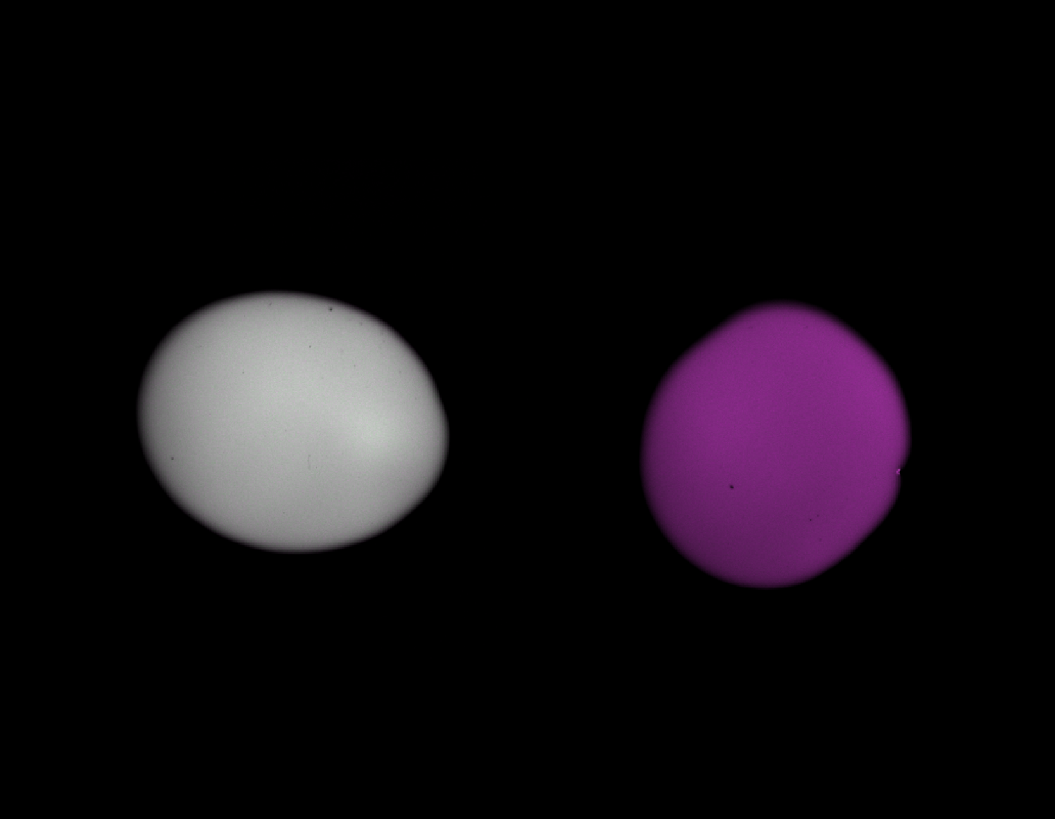
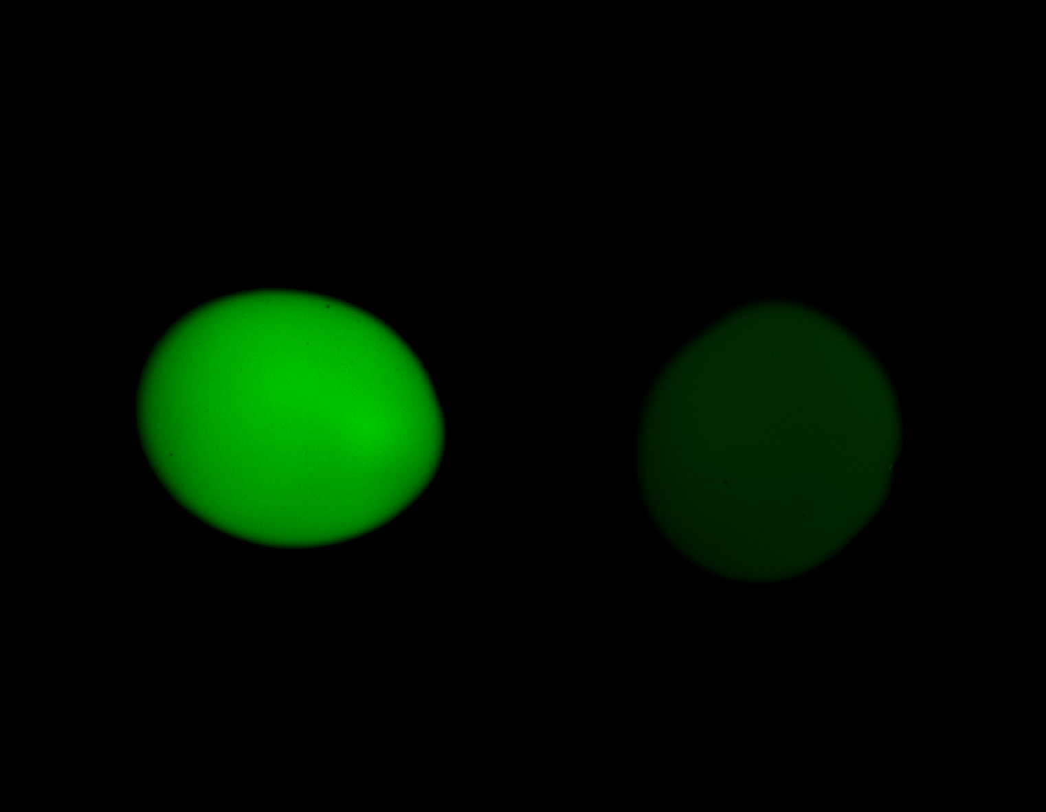
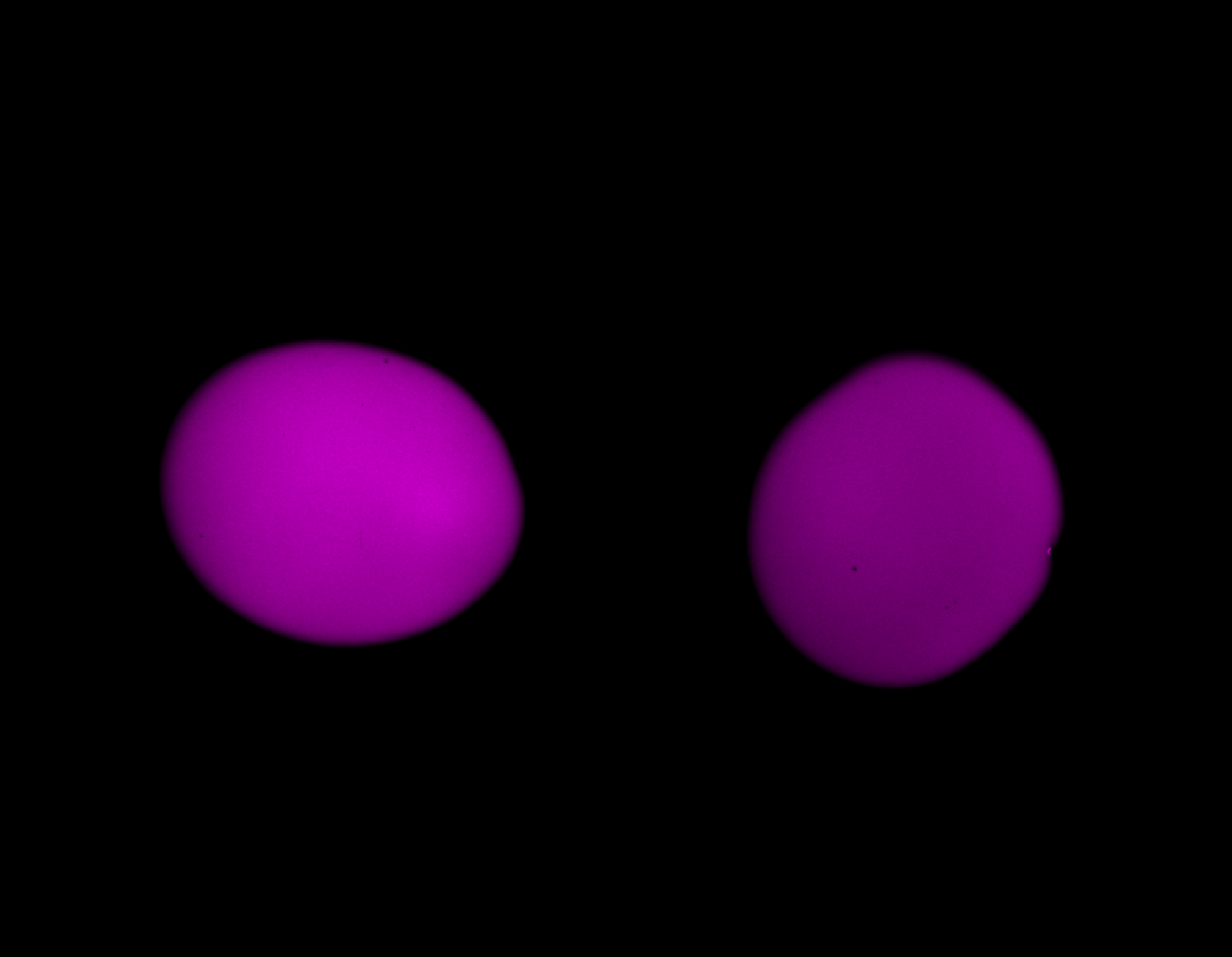
Unlike in the previous one-way unmixing example, here both channels contain bleed-through
from the other channel. Top shows the composite view of the raw synthetic stack; center and
bottom show the individual channels. spectral_unmixing offers a bidirectional workflow to
correct both channels simultaneously. The forward and reverse coefficients can be set manually
or estimated from single-label controls.
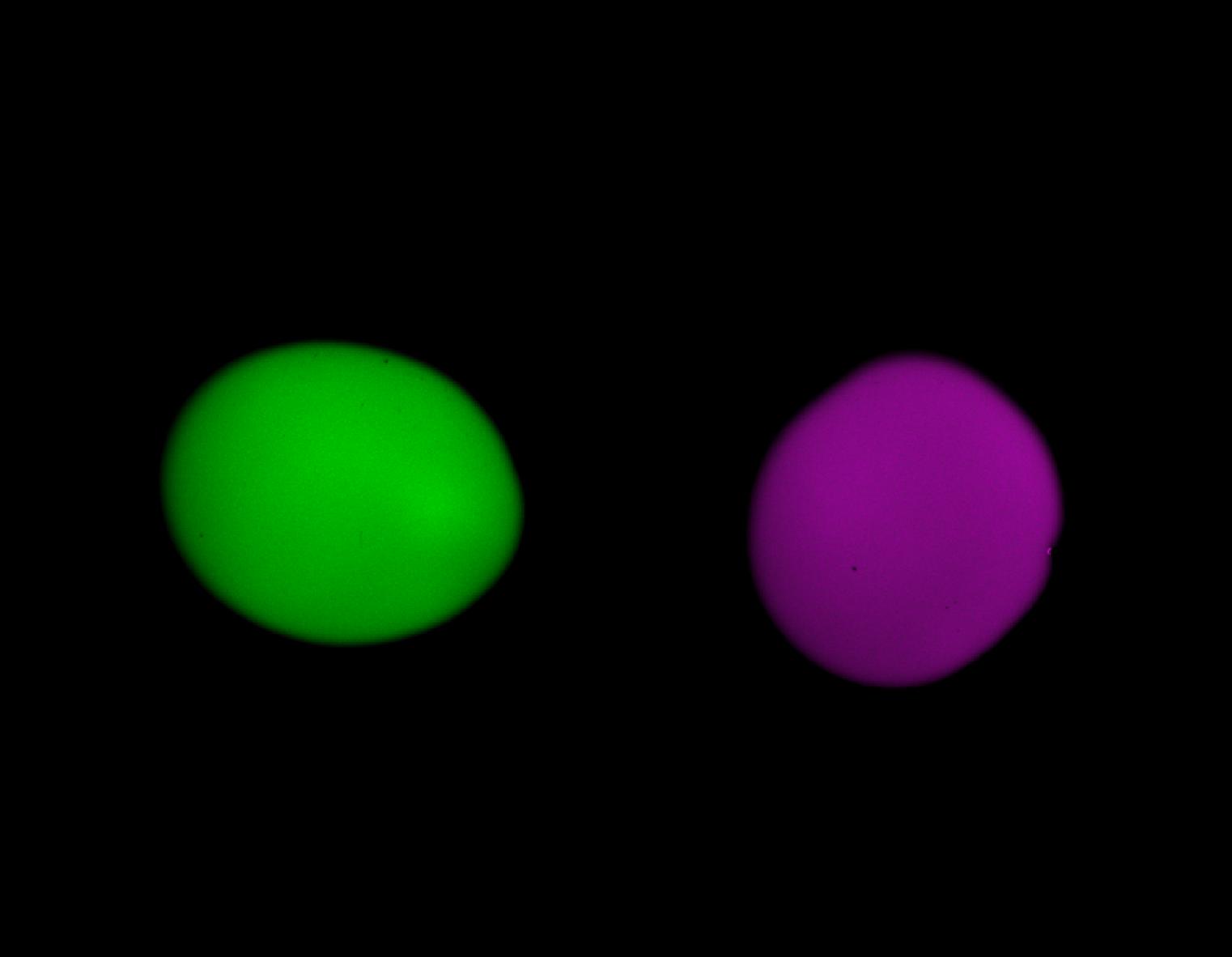


Results of the fixed bidirectional unmixing. The forward and reverse coefficients were set manually to 0.6 and 0.5, respectively. The bleed-through in both channels is effectively removed. The subsequent examples show how to estimate these coefficients automatically from the data, always resulting in a similar final output (and therefore omitted here for brevity).
Bidirectional mean_ratio
OUTPUT_REFERENCE = OUTPUT_DIR / "bidirectional_unmixed_reference_t0_mean_ratio.tif"

reference_output = unmix(
    input_path=INPUT_PATH,
    output_path=OUTPUT_REFERENCE,
    bidirectional=True,
    # source_channel=0,  # default: 0
    # target_channel=1,  # default: 1
    # alpha_mode="reference_t",
    # alpha_reference_t=0,
    method="mean_ratio",
    signal_percentile=50.0,
    background_percentile=1.0,
    # target_low_percentile=95.0,
    # preprocess_alpha_inputs=True,  # default: True
    # max_alpha_voxels=500_000,  # default
    # random_state=0,  # default
    # alpha_reverse=None,
    # method_reverse="mean_ratio",
    # signal_percentile_reverse=99.0,
    # background_percentile_reverse=0.5,
    # target_low_percentile_reverse=95.0,
)
print(reference_output)
print(report_path_from_output_path(reference_output).read_text(encoding="utf-8"))
show_unmixed_channels_in_napari(
    reference_output,
    source_channel=0,
    target_channel=1,
    layer_prefix="Bidirectional reference mean_ratio")
The most important settings are:
signal_percentile: controls how selective the forward-direction source mask is. Higher values keep only brighter source voxels; lower values include more voxels.background_percentile: controls the percentile-based background subtraction used before estimation. Higher values remove more baseline; lower values preserve more low signal.optional
target_low_percentilethe commented
*_reverseparameters if the reverse direction should use a different mask or method
This is usually the easiest automatic bidirectional mode to start with because all reverse-direction settings inherit the forward values unless you override them explicitly.
Note
The bidirectional workflow generally accepts a different estimation method.
If you want to use a different method in the reverse direction, you can set
method_reverse to one of the supported methods. If it is left at None
or omitted, the reverse direction will inherit the forward method. The same inheritance
applies to other parameters as well.
The example script shown here uses a stack with only one time point, so
alpha_mode and alpha_reference_t are left commented out in the code. For
real multi-time-point stacks, you would usually
set alpha_mode="reference_t" explicitly when one shared coefficient per
direction should be estimated from a chosen reference time point, or
alpha_mode="per_t" when one forward and one reverse coefficient should be
estimated separately for each time point. In these cases, additional relevant parameters
are:
alpha_mode:reference_torper_tfor multi-time-point stacks. The former estimates one alpha from the reference time point; the latter estimates one alpha per time point. In the presentT=1example, these arguments are commented out because the defaultreference_tbehavior witht=0is already sufficient.alpha_reference_t: defines the reference time point from which both directional coefficients are estimated. Only relevant whenalpha_mode="reference_t".
Bidirectional linear_fit
OUTPUT_REFERENCE_LINEAR_FIT = OUTPUT_DIR / "bidirectional_unmixed_reference_t0_linear_fit.tif"

reference_linear_fit_output = unmix(
    input_path=INPUT_PATH,
    output_path=OUTPUT_REFERENCE_LINEAR_FIT,
    bidirectional=True,
    # source_channel=0,  # default: 0
    # target_channel=1,  # default: 1
    method="linear_fit",
    #alpha_mode="reference_t",
    #alpha_reference_t=0,
    signal_percentile=50.0,
    background_percentile=1.0,
    # target_low_percentile=95.0,
    # preprocess_alpha_inputs=True,  # default: True
    # max_alpha_voxels=500_000,  # default
    # random_state=0,  # default
    # alpha_reverse=None,
    # method_reverse="linear_fit",
    # signal_percentile_reverse=98.0,
    # background_percentile_reverse=1.0,
    # target_low_percentile_reverse=None,
)
print(reference_linear_fit_output)
print(report_path_from_output_path(reference_linear_fit_output).read_text(encoding="utf-8"))
show_unmixed_channels_in_napari(
    reference_linear_fit_output,
    source_channel=0,
    target_channel=1,
    layer_prefix="Bidirectional reference linear_fit")
This variant estimates forward and reverse coefficients with masked least squares.
The most relevant settings are:
signal_percentilebackground_percentileoptional
target_low_percentileoptional
method_reverseoptional reverse-direction mask parameters such as
signal_percentile_reverse
This is a good choice when you want a fit-based estimate in both directions but still want to retain the same reference-time-point logic.
Bidirectional corr_min
OUTPUT_REFERENCE_CORR_MIN = OUTPUT_DIR / "bidirectional_unmixed_reference_t0_corr_min.tif"

reference_corr_min_output = unmix(
    input_path=INPUT_PATH,
    output_path=OUTPUT_REFERENCE_CORR_MIN,
    bidirectional=True,
    # source_channel=0,  # default: 0
    # target_channel=1,  # default: 1
    method="corr_min",
    # alpha_mode="reference_t",
    # alpha_reference_t=0,
    signal_percentile=50.0,
    background_percentile=1.0,
    alpha_max=1.0,
    # target_low_percentile=95.0,
    # preprocess_alpha_inputs=True,  # default: True
    # max_alpha_voxels=500_000,  # default
    # random_state=0,  # default
    # alpha_reverse=None,
    # method_reverse="corr_min",
    # signal_percentile_reverse=99.0,
    # background_percentile_reverse=1.0,
    # target_low_percentile_reverse=None,
    # alpha_max_reverse=0.5,
)
print(reference_corr_min_output)
print(report_path_from_output_path(reference_corr_min_output).read_text(encoding="utf-8"))
show_unmixed_channels_in_napari(
    reference_corr_min_output,
    source_channel=0,
    target_channel=1,
    layer_prefix="Bidirectional reference corr_min",)
Here the forward and reverse coefficients are chosen by minimizing residual correlation after correction.
The settings most worth tuning are:
alpha_max: upper bound for the forward optimization. Larger values allow stronger subtraction; smaller values keep the fit more conservative.optional
alpha_max_reversesignal_percentilebackground_percentileoptional
method_reverse
This can be more aggressive than ratio- or fit-based estimation, especially when the two channels are themselves biologically correlated.
Bidirectional mi_min
OUTPUT_REFERENCE_MI_MIN = OUTPUT_DIR / "bidirectional_unmixed_reference_t0_mi_min.tif"

reference_mi_min_output = unmix(
    input_path=INPUT_PATH,
    output_path=OUTPUT_REFERENCE_MI_MIN,
    bidirectional=True,
    # source_channel=0,  # default: 0
    # target_channel=1,  # default: 1
    method="mi_min",
    # alpha_mode="reference_t",
    # alpha_reference_t=0,
    signal_percentile=50.0,
    background_percentile=1.0,
    alpha_max=1.0,
    mi_bins=64,
    # target_low_percentile=95.0,
    # preprocess_alpha_inputs=True,  # default: True
    # max_alpha_voxels=500_000,  # default
    # random_state=0,  # default
    # alpha_reverse=None,
    # method_reverse="mi_min",
    # signal_percentile_reverse=99.0,
    # background_percentile_reverse=1.0,
    # target_low_percentile_reverse=None,
    # alpha_max_reverse=1.0,
    # mi_bins_reverse=32,
)
print(reference_mi_min_output)
print(report_path_from_output_path(reference_mi_min_output).read_text(encoding="utf-8"))
show_unmixed_channels_in_napari(
    reference_mi_min_output,
    source_channel=0,
    target_channel=1,
    layer_prefix="Bidirectional reference mi_min")
This method uses the two-channel PICASSO-like mutual-information criterion in both directions.
The key settings are:
mi_bins: histogram resolution for the mutual-information objective. Higher values can capture finer structure but can become less stable; lower values are coarser and often more robust.optional
mi_bins_reversealpha_maxoptional
alpha_max_reversemask and preprocessing settings for each direction
This is the most flexible of the scalar bidirectional estimators, but also the slowest and potentially the most aggressive if the channels are biologically linked.
What to tune most often
For real bidirectional datasets, the most important additional controls beyond the standard one-way workflow are:
alpha_reversemethod_reversesignal_percentile_reversebackground_percentile_reversetarget_low_percentile_reversealpha_max_reversemi_bins_reverse
Any reverse parameter left at None falls back to the corresponding forward
setting. That inheritance model is convenient for a first pass, but for real
data it is often worth checking whether the reverse direction deserves its own
masking or optimization settings.